
Unlocking Optimal Routes: Navigating the Labyrinth of TSP Algorithms
Explore the diverse landscape of algorithms designed to tackle the Traveling Salesman Problem, from simple heuristics to advanced optimization techniques.
Key Highlights of TSP Algorithms
- Heuristics: Approximate solutions like Nearest Neighbor and Clarke-Wright offer quick, practical routes, especially for large-scale problems.
- Optimization Techniques: Methods such as Simulated Annealing and Genetic Algorithms refine initial solutions for near-optimal results by iteratively improving the route.
- Exact Algorithms: While computationally intensive, approaches like Dynamic Programming guarantee the shortest possible route, suitable for smaller problem instances.
Understanding the Traveling Salesman Problem (TSP)
The Traveling Salesman Problem (TSP) is a classic problem in combinatorial optimization. It asks the following question: "Given a list of cities and the distances between each pair of cities, what is the shortest possible route that visits each city exactly once and returns to the origin city?" Despite its simple formulation, the TSP is notoriously difficult to solve, especially as the number of cities increases. This difficulty stems from the fact that the number of possible routes grows factorially with the number of cities, making an exhaustive search impractical for even moderately sized problems.
The TSP is an NP-hard problem, meaning that no polynomial-time algorithm is known to solve it optimally. This has led to the development of a wide range of algorithms, from exact methods that guarantee the optimal solution (but are only feasible for small problem instances) to heuristics and approximation algorithms that provide good, but not necessarily optimal, solutions in a reasonable amount of time. These algorithms find applications across various fields, including logistics, transportation, manufacturing, and circuit design.
Why is TSP so Widely Studied?
The TSP serves as a benchmark for new optimization techniques and algorithms. Its widespread study is due to its:
- Practical Relevance: Many real-world problems can be modeled as a TSP or a variant thereof.
- Computational Challenge: The TSP's NP-hardness makes it a challenging problem to solve, pushing the boundaries of algorithm design and optimization techniques.
- Theoretical Significance: The TSP is closely related to other important problems in computer science and operations research, making it a valuable tool for studying the limits of computation.
Categories of TSP Algorithms
TSP algorithms can be broadly categorized into exact algorithms, heuristics, and metaheuristics. Each category offers a different trade-off between solution quality and computational cost.
Exact Algorithms
Exact algorithms guarantee finding the optimal solution to the TSP. However, their computational complexity makes them impractical for large problem instances. Some common exact algorithms include:
- Brute Force: This involves checking all possible routes, which is only feasible for very small problems due to its exponential time complexity.
- Dynamic Programming: This approach breaks the problem down into smaller subproblems, solving each subproblem only once and storing the results in a table. The Held-Karp algorithm is a well-known dynamic programming algorithm for the TSP.
- Branch and Bound: This algorithm systematically searches the solution space, pruning branches that cannot lead to the optimal solution. It requires a good lower bound on the optimal tour length to be effective.
Heuristics
Heuristics are algorithms that provide good, but not necessarily optimal, solutions in a reasonable amount of time. They are often used for large problem instances where exact algorithms are not feasible. Some common heuristics for the TSP include:
- Nearest Neighbor: This algorithm starts at a random city and repeatedly visits the nearest unvisited city until all cities have been visited.
- Insertion Heuristics: These algorithms start with a small tour and gradually insert the remaining cities into the tour. Common insertion heuristics include:
- Convex Hull Insertion: Cities are added based on their proximity to the convex hull of the existing tour.
- Cheapest Insertion: The city that can be inserted into the tour with the least increase in tour length is added.
- Minimum Spanning Tree (MST) based heuristics: These algorithms build a minimum spanning tree of the cities and then traverse the tree to create a tour. Christofides algorithm is a well-known MST-based heuristic that guarantees a solution within 1.5 times the optimal.
- Clarke-Wright Algorithm (Savings Heuristic): This algorithm starts with each city on its own separate route back to the depot and then iteratively merges the two routes that offer the greatest savings in distance.
Metaheuristics
Metaheuristics are high-level problem-solving strategies that guide the search process to find near-optimal solutions. They often involve exploring the solution space in a more intelligent way than simple heuristics. Some common metaheuristics for the TSP include:
-
Simulated Annealing: This algorithm is inspired by the annealing process in metallurgy. It starts with a random solution and gradually improves it by making small changes. The algorithm accepts both improving and worsening moves, with the probability of accepting a worsening move decreasing as the "temperature" decreases.
-
Genetic Algorithms: These algorithms are inspired by the process of natural selection. They start with a population of random solutions and then iteratively improve the population by applying genetic operators such as crossover and mutation.
-
Tabu Search: This algorithm explores the solution space by iteratively moving from one solution to a neighboring solution. To avoid cycling, the algorithm maintains a tabu list of recently visited solutions that cannot be revisited.
-
Ant Colony Optimization: Inspired by the foraging behavior of ants, this algorithm uses a colony of artificial ants to search for good solutions. The ants deposit pheromones on the edges they traverse, and the pheromone levels guide the search process.
-
Neural Networks: Self-Organizing Maps (SOM), also known as Kohonen maps, are used to reduce the dimensionality of data. In the context of TSP, they can help in clustering cities and finding a near-optimal route by organizing the cities in a topologically meaningful way.
-
Bee Colony Optimization: This algorithm mimics the foraging behavior of honeybees to find optimal solutions. In the context of TSP, artificial bees explore different routes and share information about the quality of their findings, leading to the discovery of shorter paths.
Visualizing TSP Heuristics
Here's a look at different TSP heuristics in action. These images help illustrate how different algorithms approach the problem of finding the shortest route.
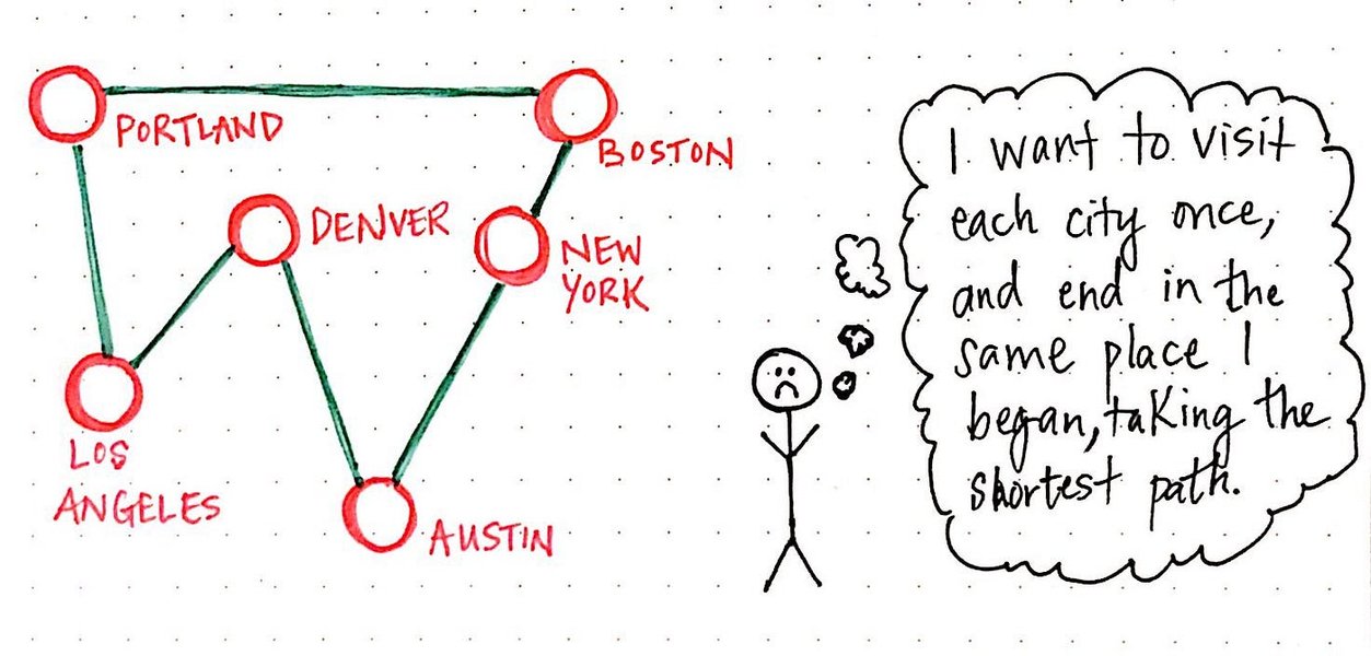
Visualization of a TSP solution path.
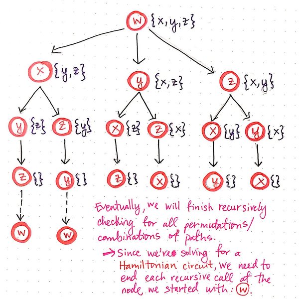
Another example of a TSP route.
Visualizing these algorithms helps in understanding their strengths and weaknesses. For instance, the Nearest Neighbor heuristic is easy to implement but often yields suboptimal results, while more complex algorithms like Simulated Annealing can find better solutions at the cost of increased computational time.
Comparative Analysis of TSP Algorithms
Choosing the right algorithm for the TSP depends on the specific requirements of the problem, including the size of the problem instance, the desired solution quality, and the available computational resources.
Algorithm Comparison Table
The following table provides a comparative analysis of some of the most common TSP algorithms:
| Algorithm | Type | Solution Quality | Computational Complexity | Advantages | Disadvantages | Suitable For |
|---|---|---|---|---|---|---|
| Brute Force | Exact | Optimal | O(n!) | Guarantees optimal solution | Only feasible for very small problems | Very small problem instances |
| Dynamic Programming (Held-Karp) | Exact | Optimal | O(n^2 * 2^n) | Guarantees optimal solution | Limited to moderately sized problems | Small to medium-sized problem instances |
| Nearest Neighbor | Heuristic | Suboptimal | O(n^2) | Simple and fast | Can produce poor solutions | Large problem instances where speed is critical |
| Christofides Algorithm | Heuristic | Within 1.5x optimal | O(n^3) | Guaranteed approximation ratio | More complex than Nearest Neighbor | Medium to large-sized problem instances |
| Simulated Annealing | Metaheuristic | Near-optimal | Varies | Can escape local optima | Requires careful tuning of parameters | Medium to large-sized problem instances |
| Genetic Algorithm | Metaheuristic | Near-optimal | Varies | Robust and can handle complex problems | Computationally intensive | Large problem instances with complex constraints |
| Clarke-Wright Algorithm | Heuristic | Suboptimal | O(n^2 log n) | Relatively simple and efficient | May not perform well on all types of problem instances | Large problem instances where a quick, reasonable solution is needed |
The Christofides Algorithm: A Detailed Look
The Christofides algorithm is a notable heuristic for the Traveling Salesman Problem, providing a solution that is guaranteed to be within 1.5 times the optimal solution. This makes it a valuable tool when near-optimal solutions are required without the computational burden of exact methods. The algorithm combines concepts from graph theory to improve upon simpler TSP heuristics.
How Christofides Algorithm Works
The Christofides algorithm involves the following steps:
- Compute the Minimum Spanning Tree (MST): Construct an MST, \( T \), for the graph \( G \) representing the TSP instance. The MST connects all vertices with the minimum possible total edge weight and can be found using algorithms like Prim's or Kruskal's.
- Identify Odd-Degree Vertices: Find the set \( O \) of vertices in \( T \) that have an odd degree (number of incident edges).
- Compute Minimum-Weight Perfect Matching: Find a minimum-weight perfect matching \( M \) on the subgraph induced by the vertices in \( O \). A perfect matching pairs each vertex in \( O \) with exactly one other vertex, such that the sum of the weights of the edges in \( M \) is minimized.
- Form a Multigraph: Combine the edges of \( T \) and \( M \) to form a multigraph \( H \). This graph may have multiple edges between vertices.
- Create an Eulerian Circuit: Since every vertex in \( H \) has an even degree, there exists an Eulerian circuit, which is a path that visits every edge exactly once. Find such a circuit in \( H \).
- Convert to TSP Tour: Transform the Eulerian circuit into a TSP tour by traversing the circuit and skipping over previously visited vertices. This step maintains the order of first visitations.
The crucial insight behind the Christofides algorithm is the use of minimum-weight perfect matching. By matching the odd-degree vertices, it ensures that we can create an Eulerian circuit, which then leads to a relatively short TSP tour.
Dynamic Programming Approach
Dynamic Programming offers a structured method to solve the TSP, ensuring an optimal solution by breaking down the problem into smaller, overlapping subproblems. This approach is particularly useful for graphs of moderate size where exact solutions are feasible.
Implementation of Dynamic Programming in TSP
The dynamic programming approach to TSP typically uses a recursive relation to find the shortest path. Let \(C(S, i)\) be the cost of the shortest path visiting each node in set \(S\) exactly once, starting at node 1 and ending at node \(i\). The recursive definition can be given as:
\[ C(S, i) = \min_{j \in S, j \neq i} \{C(S - \{i\}, j) + d_{ji}\} \]Where \(d_{ji}\) is the distance from node \(j\) to node \(i\). The base case is when \(S = \{1, i\}\), the cost is simply the distance \(d_{1i}\).
Here's a step-by-step breakdown:
- Define Subproblems: The subproblems are defined as finding the shortest path from the starting city to another city, visiting each intermediate city only once.
- Establish Recurrence Relation: The optimal solution is constructed from the solutions of the subproblems. The recurrence relation calculates the minimum cost to reach a city from the starting city via all possible subsets of other cities.
- Compute Solutions: The solutions to the subproblems are computed and stored in a table. This avoids recomputation and reduces time complexity.
- Construct Optimal Solution: The final solution is constructed by combining the solutions to the subproblems, resulting in the shortest possible route.
Dynamic Programming ensures each subproblem is solved only once, significantly reducing the computational effort compared to brute-force methods.
Heuristics in Action: A Nearest Neighbor Example
The Nearest Neighbor algorithm is one of the simplest heuristics for the TSP. It constructs a tour by starting at an arbitrary city and then repeatedly visiting the nearest unvisited city until all cities have been visited.
Illustrative Example
Consider a scenario with five cities (A, B, C, D, E) and the following distance matrix:
\[ \begin{bmatrix} 0 & 10 & 15 & 20 & 25 \\ 10 & 0 & 35 & 25 & 30 \\ 15 & 35 & 0 & 30 & 40 \\ 20 & 25 & 30 & 0 & 15 \\ 25 & 30 & 40 & 15 & 0 \end{bmatrix} \]Starting from city A, the Nearest Neighbor algorithm would proceed as follows:
- Start at A: Current tour: A
- Nearest to A: City B (distance 10). Current tour: A → B
- Nearest to B (excluding A): City D (distance 25). Current tour: A → B → D
- Nearest to D (excluding A, B): City E (distance 15). Current tour: A → B → D → E
- Last city: City C. Current tour: A → B → D → E → C
- Return to A: Final tour: A → B → D → E → C → A
The total distance of this tour is 10 + 25 + 15 + 40 + 15 = 105.
While simple to implement, the Nearest Neighbor algorithm often yields suboptimal solutions. The quality of the solution heavily depends on the starting city and the structure of the problem instance.
Refining Solutions with the 2-Opt Heuristic
The 2-Opt heuristic is a local search algorithm used to improve existing TSP tours by iteratively swapping pairs of edges in the tour. This method can be applied to any initial tour, regardless of how it was constructed, making it a versatile tool for refining solutions.
How 2-Opt Works
The basic idea behind 2-Opt is to take a tour and systematically check if replacing two edges with two different edges would shorten the tour. If it does, the swap is made, and the process continues until no further improvements can be found.
Given a tour \([v_1, v_2, ..., v_n]\), the 2-Opt procedure involves the following steps:
- Select Two Edges: Choose two edges, \((v_i, v_{i+1})\) and \((v_j, v_{j+1})\), from the tour.
- Swap and Reverse: Remove these edges and replace them with edges \((v_i, v_j)\) and \((v_{i+1}, v_{j+1})\). This reverses the portion of the tour between \(v_{i+1}\) and \(v_j\).
- Check for Improvement: Calculate the change in tour length resulting from the swap. If the new tour is shorter, accept the swap.
- Repeat: Continue this process until no further improvements can be found.
Mathematically, the condition for accepting the swap is:
\[ d(v_i, v_{i+1}) + d(v_j, v_{j+1}) > d(v_i, v_j) + d(v_{i+1}, v_{j+1}) \]Where \(d(v_i, v_j)\) is the distance between vertices \(v_i\) and \(v_j\).
The 2-Opt heuristic is effective at removing crossing edges, which are a common source of inefficiency in TSP tours.
YouTube Deep Dive: Approximation Algorithms for TSP
This video explains approximation algorithms for solving the Traveling Salesman Problem in polynomial time, focusing on practical approaches for finding efficient routes.
Approximation algorithms are crucial for tackling the TSP, especially in scenarios where finding the absolute optimal solution is computationally infeasible. These algorithms aim to find a solution within a guaranteed factor of the optimal solution in polynomial time. The video likely covers techniques such as the Minimum Spanning Tree (MST) heuristic and Christofides algorithm, which provide solutions within a known approximation ratio.
Understanding these algorithms is essential for practitioners who need to find reasonably good solutions to the TSP quickly, making them a valuable addition to the toolkit of any operations researcher or computer scientist.
Frequently Asked Questions (FAQ)
References
Last updated April 10, 2025