Unveiling the Essence of Limits: A Cornerstone of Calculus

In the vast landscape of mathematics, the concept of a "limit" stands as a foundational pillar, particularly within the realm of calculus. It’s not just an abstract idea; it's a powerful tool that allows us to understand the behavior of functions and sequences as they approach specific values or infinity. Rather than simply evaluating a function at a point, limits illuminate what happens in the immediate vicinity of that point, even if the function itself isn't defined there.

Key Insights into Limits

Fundamental to Calculus: Limits are the bedrock upon which continuity, derivatives, and integrals are built, making them indispensable for understanding rates of change and accumulation.
Behavior Near a Point: A limit describes the value a function "approaches" as its input gets infinitesimally close to a particular value, not necessarily the value of the function at that exact point.
Beyond Direct Substitution: While direct substitution often works, limits are crucial for handling indeterminate forms (like 0/0) where direct calculation is impossible, requiring algebraic manipulation or advanced rules.

Defining the Limit: A Mathematical Journey

At its core, a limit in mathematics is the value that a function (or sequence) gets arbitrarily close to as its input (or index) approaches some specified value. This concept is crucial for understanding the behavior of functions, especially at points where they might be undefined or exhibit unusual behavior. The formal definition of a limit, often referred to as the epsilon-delta definition, was formalized by Augustin-Louis Cauchy and Karl Weierstrass in the 19th century. This precise definition allows mathematicians to rigorously prove theorems and establish the fundamental concepts of calculus.

The Intuitive Understanding of a Limit

Imagine a function $$f(x)$$ and a specific point $$a$$ on the x-axis. As $$x$$ gets closer and closer to $$a$$ (from either the left or the right), the value of $$f(x)$$ approaches a particular value, let's call it $$L$$ . This value $$L$$ is the limit of the function as $$x$$ approaches $$a$$ . It's important to note that the limit doesn't care what happens exactly at $$x = a$$ ; it only concerns the behavior of the function around that point. For instance, the function might have a hole at $$x = a$$ , or its value at $$a$$ might be different from the limit.

Consider the function $f(x) = \frac{x^2 - 1}{x - 1}$ . This function is undefined at $$x = 1$$ because it leads to division by zero. However, if we simplify the expression, we get $f(x) = \frac{(x-1)(x+1)}{x-1} = x+1$ for $x \neq 1$ . As $$x$$ approaches 1, $$f(x)$$ approaches $$1+1=2$$ . So, the limit of this function as $$x$$ approaches 1 is 2, even though the function itself is not defined at $$x=1$$ .

The Formal Epsilon-Delta Definition

The rigorous definition of a limit, often denoted as $\lim_{x \to a} f(x) = L$ , states:

Let $$f(x)$$ be defined for all $x \neq a$ over an open interval containing $$a$$ . Let $$L$$ be a real number. Then $\lim_{x \to a} f(x) = L$ if, for every $\epsilon > 0$ , there exists a $\delta > 0$ , such that if $0 < |x - a| < \delta$ , then $|f(x) - L| < \epsilon$ .

This definition might seem daunting, but it essentially means that we can make the function's output $$f(x)$$ as close to $$L$$ as we desire (within $\epsilon$ distance), simply by choosing $$x$$ sufficiently close to $$a$$ (within $\delta$ distance), without necessarily being equal to $$a$$ .

Types of Limits

Limits can be classified based on how the input variable approaches a certain value, or if it approaches infinity.

One-Sided Limits

One-sided limits consider the behavior of a function as the input approaches a point from a specific direction:

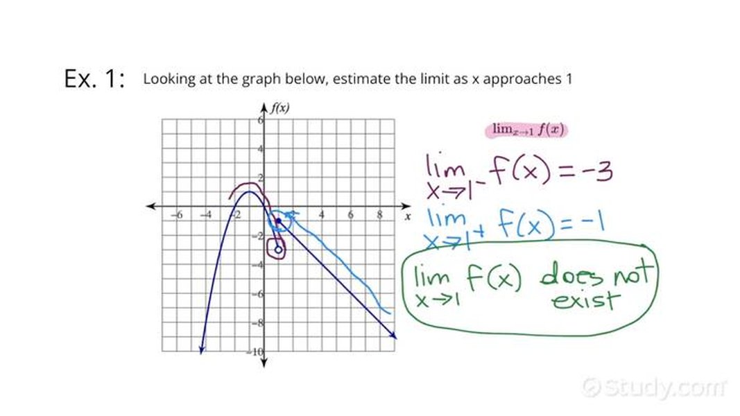
Left-Hand Limit: Denoted as $\lim_{x \to a^-} f(x)$ , this describes the value $$f(x)$$ approaches as $$x$$ gets closer to $$a$$ from values less than $$a$$ .
Right-Hand Limit: Denoted as $\lim_{x \to a^+} f(x)$ , this describes the value $$f(x)$$ approaches as $$x$$ gets closer to $$a$$ from values greater than $$a$$ .

For a two-sided limit $\lim_{x \to a} f(x)$ to exist, both the left-hand limit and the right-hand limit must exist and be equal.

Limits at Infinity

Limits at infinity describe the behavior of a function as its input grows infinitely large (positive or negative). These limits are crucial for understanding horizontal asymptotes and the long-term behavior of functions.

$\lim_{x \to \infty} f(x) = L$ : The function approaches a finite value $$L$$ as $$x$$ becomes very large.
$\lim_{x \to -\infty} f(x) = L$ : The function approaches a finite value $$L$$ as $$x$$ becomes very small (large negative).
Infinite Limits at Infinity: $\lim_{x \to \infty} f(x) = \infty$ or $\lim_{x \to \infty} f(x) = -\infty$ (and similarly for $x \to -\infty$ ). This means the function grows without bound as $$x$$ approaches infinity.

Methods for Computing Limits

Calculating limits involves various techniques, depending on the form of the function and the point being approached. Here are some common methods:

Direct Substitution

For many well-behaved functions (polynomials, rational functions where the denominator is non-zero at the limit point, trigonometric functions, etc.), the limit can be found by simply substituting the value $$a$$ into the function.

Example: $\lim_{x \to 2} (x^2 + 3x - 1) = (2)^2 + 3(2) - 1 = 4 + 6 - 1 = 9$ .

Algebraic Manipulation

When direct substitution results in an indeterminate form (like $\frac{0}{0}$ or $\frac{\infty}{\infty}$ ), algebraic techniques are often necessary:

Factoring: Useful for rational functions where a common factor can be cancelled.


\(\lim_{x \to 3} \frac{x^2 - 9}{x - 3} = \lim_{x \to 3} \frac{(x-3)(x+3)}{x - 3} = \lim_{x \to 3} (x+3) = 3+3 = 6\)

Rationalizing (Conjugates): Employed when functions involve square roots.


\(\lim_{x \to 0} \frac{\sqrt{x+1} - 1}{x} = \lim_{x \to 0} \frac{\sqrt{x+1} - 1}{x} \cdot \frac{\sqrt{x+1} + 1}{\sqrt{x+1} + 1}\)
\(= \lim_{x \to 0} \frac{(x+1) - 1}{x(\sqrt{x+1} + 1)} = \lim_{x \to 0} \frac{x}{x(\sqrt{x+1} + 1)}\)
\(= \lim_{x \to 0} \frac{1}{\sqrt{x+1} + 1} = \frac{1}{\sqrt{0+1} + 1} = \frac{1}{1+1} = \frac{1}{2}\)

Common Denominators: For expressions involving fractions.

L'Hôpital's Rule

L'Hôpital's Rule is a powerful technique applicable to limits of the form $\frac{0}{0}$ or $\frac{\infty}{\infty}$ . It states that if $\lim_{x \to a} \frac{f(x)}{g(x)}$ is an indeterminate form, then $\lim_{x \to a} \frac{f(x)}{g(x)} = \lim_{x \to a} \frac{f'(x)}{g'(x)}$ , provided the latter limit exists. This involves taking the derivatives of the numerator and denominator separately.

Squeeze Theorem (Sandwich Theorem)

The Squeeze Theorem is useful when direct evaluation or algebraic manipulation is difficult. If $g(x) \le f(x) \le h(x)$ for all $$x$$ in an open interval containing $$a$$ (except possibly at $$a$$ ), and if $\lim_{x \to a} g(x) = L$ and $\lim_{x \to a} h(x) = L$ , then $\lim_{x \to a} f(x) = L$ .

Numerical and Graphical Approaches

Limits can also be estimated numerically by evaluating the function at values increasingly close to the point of interest, or graphically by observing the function's behavior on a graph. Online calculators like Desmos and Wolfram|Alpha can assist in visualizing limits and providing step-by-step solutions.

Demonstration of using Desmos Graphing Calculator to investigate limits via graphs and tables.

Properties and Laws of Limits

Limits adhere to several fundamental properties and laws that simplify their calculation and application:

Property/Law	Description	Mathematical Notation
Constant Rule	The limit of a constant is the constant itself.	$\lim_{x \to a} c = c$
Identity Rule	The limit of $$x$$ as $$x$$ approaches $$a$$ is $$a$$ .	$\lim_{x \to a} x = a$
Sum Rule	The limit of a sum is the sum of the limits.	$\lim_{x \to a} [f(x) + g(x)] = \lim_{x \to a} f(x) + \lim_{x \to a} g(x)$
Difference Rule	The limit of a difference is the difference of the limits.	$\lim_{x \to a} [f(x) - g(x)] = \lim_{x \to a} f(x) - \lim_{x \to a} g(x)$
Constant Multiple Rule	The limit of a constant times a function is the constant times the limit of the function.	$\lim_{x \to a} [c \cdot f(x)] = c \cdot \lim_{x \to a} f(x)$
Product Rule	The limit of a product is the product of the limits.	$\lim_{x \to a} [f(x) \cdot g(x)] = \lim_{x \to a} f(x) \cdot \lim_{x \to a} g(x)$
Quotient Rule	The limit of a quotient is the quotient of the limits, provided the limit of the denominator is not zero.	$\lim_{x \to a} \frac{f(x)}{g(x)} = \frac{\lim_{x \to a} f(x)}{\lim_{x \to a} g(x)}$ , if $\lim_{x \to a} g(x) \neq 0$
Power Rule	The limit of a function raised to a power is the limit of the function raised to that power.	$\lim_{x \to a} [f(x)]^n = [\lim_{x \to a} f(x)]^n$

The Significance of Limits in Calculus and Beyond

Limits are not merely a theoretical construct; they have profound implications across various fields of mathematics and science.

Continuity

A function is considered continuous at a point if its limit at that point exists, the function is defined at that point, and the limit value equals the function's value at that point. Without limits, the rigorous definition of continuity would be impossible.

Graph showing a function with a hole, illustrating a limit concept.

An illustrative graph demonstrating a function with a discontinuity where a limit might still exist.

Derivatives

The derivative of a function, which represents its instantaneous rate of change or the slope of the tangent line to its graph at a given point, is formally defined using a limit:

\[ \frac{df}{dx} = f'(x) = \lim_{h \to 0} \frac{f(x+h) - f(x)}{h} \]

This definition highlights how derivatives essentially measure the limit of average rates of change over infinitesimally small intervals.

Integrals

Definite integrals, which represent the area under a curve, are also defined using limits. Specifically, they are the limit of Riemann sums as the width of the rectangles used to approximate the area approaches zero.

\[ \int_a^b f(x) \, dx = \lim_{n \to \infty} \sum_{i=1}^n f(x_i^*) \Delta x \]

This demonstrates how limits allow us to transition from discrete approximations to continuous quantities.

Real-World Applications

While often abstract, limits appear in many real-world scenarios:

Physics: Calculating instantaneous velocity from average velocity, or understanding the behavior of physical systems as conditions approach certain extremes.
Economics: Analyzing marginal costs and revenues, or understanding how economic models behave as variables approach certain thresholds.
Engineering: Designing systems where variables need to approach a target value without overshooting, or predicting the long-term behavior of processes.

Complexity and Challenge in Limit Problems

Solving limit problems can range from straightforward direct substitution to complex algebraic manipulation and the application of advanced theorems. The difficulty often lies in recognizing the appropriate technique for indeterminate forms or understanding piecewise functions.

This radar chart illustrates the perceived complexity and required skills for tackling different types of limit problems. Basic limit problems primarily rely on direct substitution and understanding fundamental limit laws, with some algebraic manipulation. Advanced problems, involving indeterminate forms that require L'Hôpital's Rule or the Squeeze Theorem, demand a deeper conceptual understanding, more sophisticated algebraic skills, and broader problem-solving versatility. Graphical interpretation remains valuable across both levels, but the emphasis shifts as problems become more analytical.

FAQ about Limits

What is a limit in mathematics?

In mathematics, a limit is the value that a function or sequence approaches as its input or index gets closer and closer to some specified value. It describes the behavior of the function in the vicinity of a point, rather than at the point itself.

Why are limits important in calculus?

Limits are fundamental to calculus because they are used to define continuity, derivatives (the rate of change of a function), and integrals (the accumulation of a quantity). Without the concept of a limit, these core calculus concepts cannot be rigorously defined.

What does it mean if a limit does not exist?

A limit does not exist if the function approaches different values from the left and right sides of the point, if the function oscillates infinitely near the point, or if the function grows without bound (approaches infinity or negative infinity) at that point.

Can a limit exist even if the function is undefined at that point?

Yes, absolutely. This is one of the key strengths of limits. The definition of a limit explicitly states that it concerns the behavior of the function *near* a point, not necessarily *at* the point. For example, a function with a hole in its graph at a specific point can still have a finite limit at that point.

Conclusion

The concept of a limit is a cornerstone of calculus, providing the mathematical framework to understand dynamic processes and the behavior of functions. From its intuitive understanding as an "approaching value" to its rigorous epsilon-delta definition, limits enable the precise formulation of continuity, derivatives, and integrals. Mastering limits is essential for anyone delving into higher mathematics, as it unlocks the ability to analyze complex functions and model real-world phenomena with unprecedented accuracy.