Understanding the 'Degree' Parameter in Polynomial Kernel SVMs

Introduction to Support Vector Machines and Polynomial Kernels

Support Vector Machines (SVMs) are powerful supervised learning models used for classification and regression tasks. Among the various kernel functions available for SVMs, the polynomial kernel is a popular choice due to its ability to model complex relationships in data by transforming it into a higher-dimensional space. The effectiveness of a polynomial kernel largely depends on its parameters, particularly the degree parameter.

Defining the Polynomial Kernel

The polynomial kernel function is mathematically defined as:

$$ K(\mathbf{x}, \mathbf{y}) = (\gamma \langle \mathbf{x}, \mathbf{y} \rangle + r)^{d} $$

Where:

• K('x', 'y'): The kernel function evaluating the similarity between two data points 'x' and 'y'.
• γ: A scaling parameter that defines the influence of the dot product.
• ⟨ 'x', 'y' ⟩: The dot product of the input feature vectors 'x' and 'y'.
• r: A constant term that allows the kernel to fit the data better.
• d: The degree parameter, which determines the degree of the polynomial.

Role of the 'Degree' Parameter

Determining the Complexity of the Decision Boundary

The degree parameter plays a crucial role in defining the complexity of the decision boundary that the SVM can create. Specifically:

• Degree 1: Equivalent to a linear kernel, resulting in a linear decision boundary.
• Degree 2: Introduces quadratic interactions between features, allowing for a quadratic decision boundary.
• Higher Degrees (e.g., 3, 4): Enable even more complex, higher-order polynomial decision boundaries that can fit intricate patterns in the data.

Impact on Model Flexibility and Overfitting

A higher degree increases the flexibility of the SVM model, enabling it to capture more complex relationships within the data. However, this increased flexibility comes with a trade-off:

• Overfitting Risk: As the degree increases, the model may become too tailored to the training data, capturing noise and reducing its ability to generalize to unseen data.
• Underfitting Risk: Conversely, a very low degree (e.g., degree 1) may lead to underfitting, where the model is too simple to capture the underlying patterns in the data.

Mathematical Interpretation of the Degree Parameter

The polynomial kernel's ability to map data into a higher-dimensional space is governed by the degree parameter. Here's a closer look at how it works:

Polynomial Expansion

The degree determines the highest power of the input features considered in the kernel function. For instance:

• Degree 2: Considers interactions like x₁², x₁x₂, x₂², etc.
• Degree 3: Includes terms like x₁³, x₁²x₂, x₁x₂², x₂³, and so forth.
• Higher Degrees: Incorporate even more complex combinations of input features.

This expansion allows the SVM to separate data points that are not linearly separable in the original feature space by finding a hyperplane in the transformed higher-dimensional space.

Choosing the Optimal Degree

Selecting the appropriate degree is pivotal for the model's performance and is often determined through a combination of domain knowledge and empirical testing.

Techniques for Optimization

• Cross-Validation: Dividing the dataset into training and validation sets to assess how different degree values affect the model's performance.
• Grid Search: Systematically exploring a range of degree values (and possibly other hyperparameters) to identify the combination that yields the best cross-validation performance.
• Automated Hyperparameter Tuning: Utilizing algorithms and tools that automate the search for optimal hyperparameters, including the degree.

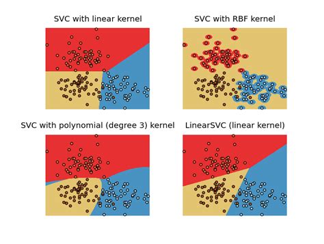
Visualizing Decision Boundaries

Visual techniques can be employed to understand how different degree values impact the decision boundaries:

• Lower Degrees: Tend to produce simpler, smoother boundaries.
• Higher Degrees: Allow for more intricate and possibly convoluted boundaries.

By visualizing these boundaries, practitioners can gain insights into whether the model is appropriately capturing the data's structure or if it's overfitting.

Considerations Based on Dataset Characteristics

The optimal degree can vary depending on:

• Data Complexity: More complex datasets may benefit from higher degree values.
• Sample Size: Smaller datasets may be prone to overfitting with higher degrees.
• Feature Interactions: If interactions between features are significant, a higher degree may better capture these relationships.

Practical Implications and Best Practices

Balancing Bias and Variance

The degree parameter influences the bias-variance trade-off in the model:

• High Degree: Low bias but high variance, leading to overfitting.
• Low Degree: High bias but low variance, leading to underfitting.

The goal is to find a degree that minimizes the generalization error by balancing these two aspects.

Regularization and Degree Selection

Incorporating regularization techniques can help mitigate overfitting when using higher degree polynomials. Regularization adds a penalty to the loss function, discouraging overly complex models:

• L1 Regularization: Encourages sparsity in feature coefficients.
• L2 Regularization: Penalizes large coefficients, promoting smoother decision boundaries.

When combined with careful degree selection, regularization can enhance the SVM's ability to generalize effectively.

Computational Considerations

Higher degree polynomials can significantly increase the computational complexity of the model:

• Training Time: More complex kernels require more computational resources and time to train.
• Memory Usage: Expanding the feature space increases memory consumption.
• Scalability: For large datasets, higher degree kernels may become impractical.

Therefore, it's essential to balance model complexity with available computational resources.

Examples and Applications

Example: Quadratic Kernel (Degree 2)

Consider a dataset where the classes are not linearly separable but can be separated by a quadratic curve. Using a polynomial kernel with degree=2 allows the SVM to create a decision boundary that captures the quadratic relationship, effectively separating the classes.

Example: Cubic Kernel (Degree 3)

In scenarios where the data requires capturing cubic relationships, a polynomial kernel with degree=3 would be appropriate. This enables the model to fit more complex patterns, though with an increased risk of overfitting.

Further Resources

For more in-depth information and practical guidance on polynomial kernels and their parameters in SVMs, consider the following resources:

Conclusion

The degree parameter in a polynomial kernel SVM is a pivotal element that dictates the complexity and flexibility of the model's decision boundary. By carefully selecting and tuning this parameter, practitioners can balance the trade-offs between underfitting and overfitting, ensuring that the SVM model generalizes well to new, unseen data. Combining an understanding of the underlying mathematics with empirical optimization techniques, such as cross-validation and grid search, facilitates the effective application of polynomial kernels in diverse machine learning tasks.