Unlocking the Cheapest Insertion Algorithm: The Intelligent Path to Optimal Routes

Key Insights

Elegant Simplicity: Cheapest Insertion builds tours incrementally by adding cities that minimize total distance increase at each step
Performance Guarantee: For symmetric TSP instances, the algorithm guarantees a tour length at most twice the optimal solution
Practical Power: Despite its simplicity, Cheapest Insertion has been used to tackle massive real-world problems with millions of locations

Understanding the Cheapest Insertion Algorithm

The Cheapest Insertion algorithm is a heuristic method designed to solve the Traveling Salesman Problem (TSP), one of the most famous problems in combinatorial optimization. The objective of TSP is to find the shortest possible route that visits each city exactly once and returns to the origin city. While finding the absolute optimal solution to TSP is computationally intensive (NP-hard), Cheapest Insertion provides a practical approach that delivers high-quality solutions efficiently.

At its core, the algorithm works by starting with a small sub-tour and gradually expanding it by inserting remaining cities one at a time. The key insight is that each new city is inserted at the position that causes the minimum increase in the overall tour length.

The Algorithm Step by Step

Initialization: Begin with a sub-tour consisting of two or three arbitrarily chosen cities.
Selection: For each city not yet in the tour, calculate the cost of inserting it between every pair of adjacent cities in the current sub-tour.
Insertion: Select the city and position that results in the minimum increase in total tour length and insert the city at that position.
Iteration: Repeat steps 2-3 until all cities have been added to the tour.

Mathematical Formulation

The cost of inserting a city r between adjacent cities i and j in the current tour is calculated as:

\[ \text{cost}(i,r,j) = c(i,r) + c(r,j) - c(i,j) \]

Where:

c(i,r) is the distance from city i to city r
c(r,j) is the distance from city r to city j
c(i,j) is the distance from city i to city j (the edge that would be removed)

The algorithm selects the city r and position (i,j) that minimizes this insertion cost.

Visual Representation of the Cheapest Insertion Process

The following radar chart compares the Cheapest Insertion algorithm with other TSP heuristic approaches across several performance dimensions. This visualization highlights the relative strengths and trade-offs of each method:

Algorithmic Characteristics

Complexity Analysis

The time complexity of the Cheapest Insertion algorithm varies based on implementation details:

Implementation Approach	Time Complexity	Space Complexity
Basic implementation	O(n²)	O(n²)
With priority queue	O(n² log n)	O(n²)
Optimized implementation	O(n²)	O(n)
Worst-case scenario	O(n³)	O(n²)

Where n represents the number of cities in the problem.

Advantages and Limitations

Advantages

Performance Guarantee: For symmetric TSP instances where distances satisfy the triangle inequality, the algorithm guarantees a tour length at most twice the optimal solution.
Practical Efficiency: The algorithm often produces high-quality solutions in practice, sometimes outperforming more complex heuristics.
Implementation Simplicity: Relatively straightforward to code and understand compared to some other TSP approaches.
Scalability: Has been successfully applied to very large instances, including problems with millions of locations.

Limitations

Non-Optimality: As a heuristic, it does not guarantee finding the absolute optimal solution.
Greedy Approach: Making locally optimal choices at each step can lead to suboptimal overall solutions.
Problem Structure Sensitivity: Performance can vary significantly depending on the specific structure of the problem instance.
Initial Tour Dependency: The quality of solutions can depend on the choice of the initial sub-tour.

Conceptual Framework of Cheapest Insertion

The following mindmap illustrates the key concepts, variations, and applications of the Cheapest Insertion algorithm:

mindmap root["Cheapest Insertion Algorithm"] ["Core Principles"] ["Incremental Tour Construction"] ["Minimizing Insertion Cost"] ["Greedy Approach"] ["2-Approximation Guarantee"] ["Algorithm Variants"] ["Standard Cheapest Insertion"] ["Convex Hull Cheapest Insertion (CHCI)"] ["Modified Cheapest Insertion"] ["Random-Start Cheapest Insertion"] ["Performance Considerations"] ["Time Complexity"] ["Space Requirements"] ["Solution Quality"] ["Scalability"] ["Applications"] ["Vehicle Routing"] ["Logistics Optimization"] ["Circuit Board Drilling"] ["Network Design"] ["Fashion Industry WIP Optimization"] ["Implementation Aspects"] ["Data Structures"] ["Distance Calculation Methods"] ["Initial Tour Selection"] ["Termination Criteria"]

Video Explanation of Insertion Heuristics

This video provides a clear demonstration of how insertion algorithms (including Cheapest Insertion) work to solve the Traveling Salesman Problem. It visualizes the process of building a tour incrementally by selecting the optimal insertion points.

The video walks through each step of the insertion process, showing how cities are selected for insertion and how the tour gradually expands until all locations have been visited. This visual explanation helps solidify understanding of the algorithm's operation.

Visual Examples of Cheapest Insertion

These images illustrate the Cheapest Insertion algorithm in action, showing how routes are constructed and optimized:

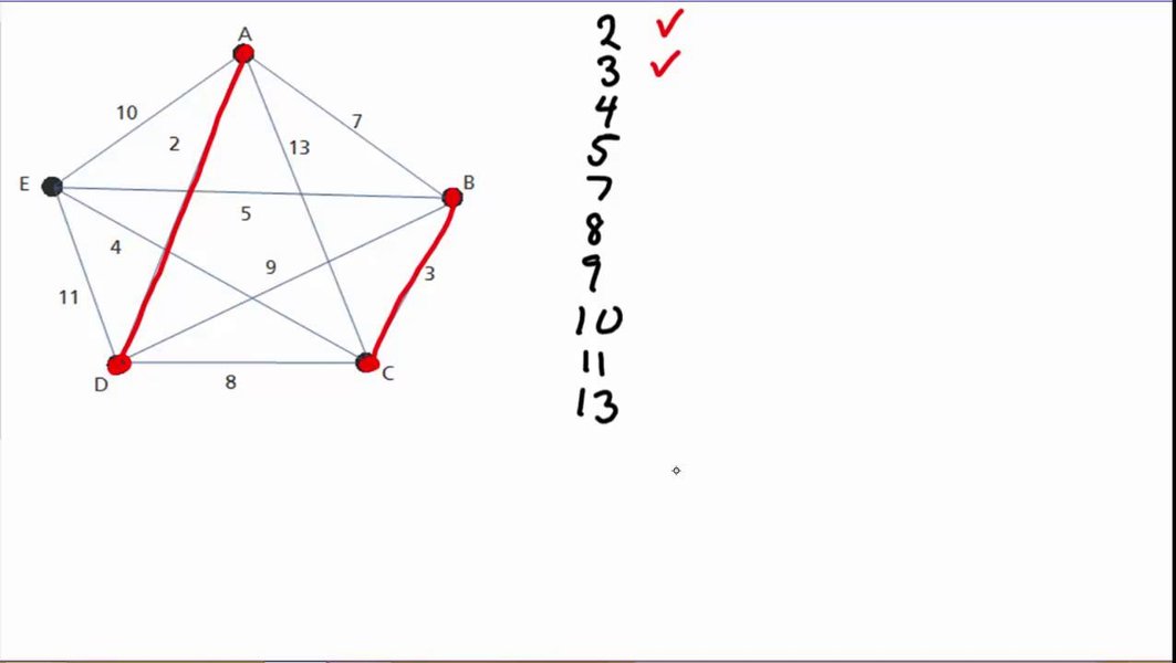
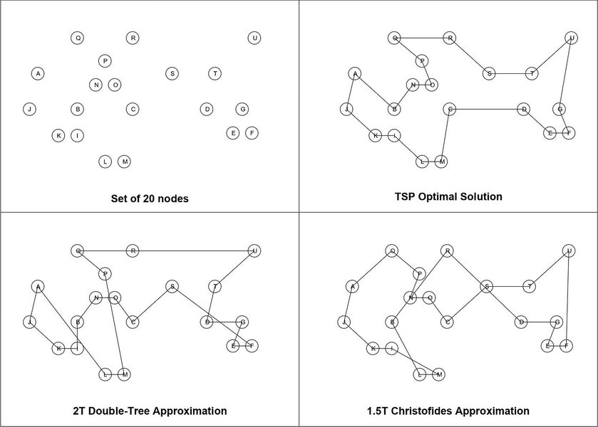
Traveling Salesman Problem Visualization

These visualizations show how the Cheapest Insertion algorithm progressively builds a tour by selecting cities based on the minimum increase in tour length. The first image demonstrates a step-by-step execution of the algorithm, while the second illustrates the resulting tour connecting multiple cities in an optimized manner.

Variations and Extensions

Common Variants

Several variations of the Cheapest Insertion algorithm have been developed to address specific needs or improve performance:

Convex Hull Cheapest Insertion (CHCI)

This variant begins by constructing a tour along the convex hull of the point set (the smallest convex polygon containing all points). The remaining interior points are then inserted using the standard cheapest insertion criteria. This approach often produces better results for geometric instances of the TSP.

Modified Cheapest Insertion

This variation starts with two strategically selected points rather than arbitrary ones, which can lead to more stable calculations for large inputs. Selection criteria for the initial points can vary, such as choosing the two most distant points.

Random-Start Cheapest Insertion

This approach uses random initial sub-tours and executes the algorithm multiple times, selecting the best resulting tour. This helps mitigate the dependency on the initial sub-tour selection.

Real-World Applications

The Cheapest Insertion algorithm has been successfully applied in various domains:

Logistics and Transportation: Route optimization for delivery vehicles and fleet management
Manufacturing: Optimizing production sequences and tool paths in automated manufacturing
Fashion Industry: Optimizing Work-In-Progress (WIP) product distributions
Circuit Board Design: Determining efficient drilling sequences for printed circuit boards
Telecommunications: Network routing and infrastructure planning

Implementation Insights

Pseudocode

function CheapestInsertion(cities):
    // Initialize with two cities (often the closest pair)
    city1, city2 = findClosestPair(cities)
    tour = [city1, city2, city1]  // Create initial sub-tour
    unvisited = cities - {city1, city2}
    
    // Main loop: insert remaining cities
    while unvisited is not empty:
        bestCost = infinity
        bestCity = null
        bestPosition = null
        
        // For each unvisited city
        for city in unvisited:
            // Try inserting between each pair of adjacent cities in tour
            for i in 0 to length(tour)-2:
                city_i = tour[i]
                city_j = tour[i+1]
                cost = distance(city_i, city) + distance(city, city_j) - distance(city_i, city_j)
                
                if cost < bestCost:
                    bestCost = cost
                    bestCity = city
                    bestPosition = i+1
        
        // Insert the city with minimum insertion cost
        tour.insert(bestPosition, bestCity)
        unvisited.remove(bestCity)
    
    return tour

Practical Implementation Tips

Distance Calculations: Pre-compute and store distances between cities in a distance matrix to avoid redundant calculations.
Data Structures: Use efficient data structures like hash sets for unvisited cities and arrays or linked lists for the tour.
Initial Tour Selection: The choice of initial sub-tour can impact solution quality. Consider starting with distant cities or using domain knowledge.
Hybrid Approaches: Consider combining Cheapest Insertion with local improvement heuristics like 2-opt or 3-opt for better results.

Frequently Asked Questions

What makes Cheapest Insertion different from other TSP heuristics?

What is the 2-approximation guarantee of Cheapest Insertion?

How does the choice of initial sub-tour affect the final solution?

Can Cheapest Insertion handle large-scale TSP problems?

How can I improve upon a Cheapest Insertion solution?