Unlocking Real-World Solutions: How Ordinary Differential Equations Shape Our Understanding

Highlights of ODE Problem-Solving

Systematic Modeling: Ordinary Differential Equations (ODEs) provide a structured framework for translating real-life dynamic problems into mathematical language, allowing for rigorous analysis.
Diverse Applications: From predicting population growth and disease spread to designing electrical circuits and understanding planetary motion, ODEs are fundamental across science, engineering, economics, and medicine.
Predictive Power: By solving ODEs, we can forecast the behavior of systems over time, understand underlying mechanisms, and make informed decisions based on quantitative insights.

The Systematic Approach: From Problem to Prediction

Applying Ordinary Differential Equations (ODEs) to solve real-life problems is a methodical process that transforms qualitative observations into quantitative, predictive models. This journey involves several key stages, ensuring that the mathematical representation accurately reflects the dynamics of the system under study.

Step 1: Defining the Real-World Challenge

Identifying the Core Problem and Variables

The initial step is to clearly articulate the real-life problem. This involves identifying the system of interest and the quantities that change over time or with respect to another independent variable. These changing quantities become the dependent variables in our model, while the variable they change with (often time) is the independent variable. For example, in studying a cooling object, the object's temperature is the dependent variable, and time is the independent variable.

Making Necessary Assumptions

Real-world systems are often incredibly complex. To make them mathematically tractable, we must make simplifying assumptions. These assumptions should be reasonable and clearly stated. For instance, when modeling simple population growth, one might initially assume unlimited resources or constant birth and death rates. The validity of these assumptions will influence the accuracy and applicability of the model.

Step 2: Crafting the Mathematical Model

Formulating the Differential Equation

Once the variables and assumptions are defined, the next step is to translate the relationships and rates of change into one or more ODEs. This involves expressing how the dependent variable(s) change with respect to the independent variable. This formulation is often based on fundamental scientific principles (e.g., Newton's laws of motion, laws of thermodynamics, chemical kinetics) or empirical observations. The order of the ODE (the highest derivative present) depends on the complexity of the interactions being modeled. For instance, the rate of cooling of an object might be proportional to the temperature difference between the object and its surroundings, leading to a first-order ODE.

Step 3: Unlocking the Solution

Classifying the ODE and Choosing a Solution Method

ODEs can be classified in various ways (e.g., linear, nonlinear, separable, homogeneous, first-order, second-order). This classification helps determine the most appropriate method for solving the equation. Some ODEs, particularly linear ones or those with simple forms, can be solved analytically. Analytical solutions provide an explicit formula for the dependent variable as a function of the independent variable. Common techniques include:

Separation of variables
Using an integrating factor (for linear first-order ODEs)
Solving characteristic equations (for linear homogeneous ODEs with constant coefficients)

However, many real-world problems lead to ODEs that are too complex for analytical solutions, especially nonlinear ODEs. In such cases, numerical methods are employed. These methods provide approximate solutions at discrete points. Popular numerical techniques include:

Euler's method
Runge-Kutta methods (e.g., RK4)

Software tools like MATLAB, Python (with libraries like SciPy and NumPy), and Mathematica are invaluable for implementing these numerical methods.

Applying Initial or Boundary Conditions

The general solution to an ODE typically contains arbitrary constants. To find a particular solution that corresponds to the specific real-life scenario, we need to apply initial conditions (values of the dependent variables and/or their derivatives at a starting point, usually t=0) or boundary conditions (values at the extremities of the domain). For example, the initial population size in a growth model or the initial temperature of a cooling object.

Step 4: Interpreting and Validating Insights

Analyzing the Solution in Context

Once a solution (analytical or numerical) is obtained, it must be interpreted in the context of the original real-world problem. This involves understanding what the mathematical results mean for the system's behavior. For instance, does the population grow indefinitely, stabilize, or decline? How quickly does an object cool? The solution allows for predictions about the future state of the system.

Model Validation and Refinement

A crucial final step is to validate the model. This involves comparing the model's predictions with real-world data or observations. If there are significant discrepancies, the model may need refinement. This could involve revisiting the initial assumptions, adding more complexity to the ODE (e.g., accounting for factors previously ignored), or using more accurate parameter values. This iterative process of modeling, solving, and validating is key to developing robust and reliable ODE-based solutions.

Visualizing ODE Concepts: A Mindmap

To better grasp the interconnectedness of the ODE problem-solving process and its diverse applications, the following mindmap illustrates the core steps and branches out to key areas where ODEs are instrumental. It shows the journey from identifying a real-world problem to applying the mathematical insights gained from the ODE model.

mindmap root["ODE Problem-Solving Lifecycle"] id1["1. Problem Identification"] id1a["Define System & Variables"] id1b["State Assumptions"] id2["2. Mathematical Formulation"] id2a["Translate to ODE(s)"] id2b["Incorporate Physical Laws / Empirical Data"] id2c["Determine Order & Type (Linear, Nonlinear)"] id3["3. Solving the ODE"] id3a["Analytical Methods"] id3aa["Separation of Variables"] id3ab["Integrating Factors"] id3ac["Characteristic Equations"] id3b["Numerical Methods"] id3ba["Euler's Method"] id3bb["Runge-Kutta Methods"] id3c["Apply Initial/Boundary Conditions"] id4["4. Interpretation & Application"] id4a["Analyze Solution Behavior"] id4b["Make Predictions"] id4c["Inform Decisions"] id5["5. Validation & Refinement"] id5a["Compare with Real Data"] id5b["Iterate on Model/Assumptions"] id6["Key Application Areas"] id6a["Physics & Engineering"] id6aa["Mechanics (Motion, Vibrations)"] id6ab["Electrical Circuits"] id6ac["Thermodynamics (Cooling)"] id6b["Biology & Medicine"] id6ba["Population Dynamics (Growth, Predator-Prey)"] id6bb["Epidemiology (Disease Spread)"] id6bc["Pharmacokinetics"] id6bd["Neuroscience (Neuronal Models)"] id6c["Economics & Finance"] id6ca["Economic Growth Models"] id6cb["Market Dynamics"] id6cc["Interest Rate Models"] id6d["Chemistry"] id6da["Reaction Kinetics"] id6db["Mixing Problems"]

This mindmap highlights the structured yet flexible nature of using ODEs. While the core steps remain consistent, the specific techniques and complexities vary greatly depending on the application domain.

Diverse Applications: ODEs in Action Across Disciplines

Ordinary Differential Equations are not just abstract mathematical constructs; they are workhorses in numerous fields, providing critical insights into how systems evolve. Below are some prominent examples illustrating their versatility.

Biology and Medicine

Population Dynamics

One of the earliest and most famous applications of ODEs is in modeling population changes. The simplest model is exponential growth, \( \frac{dP}{dt} = rP \), where \( P \) is the population, \( t \) is time, and \( r \) is the growth rate. This applies to situations with unlimited resources. A more realistic model is the logistic growth equation, \( \frac{dP}{dt} = rP(1 - \frac{P}{K}) \), which includes a carrying capacity \( K \), representing resource limitations. These models are vital for ecology, conservation, and resource management. Systems of ODEs, like the Lotka-Volterra equations, model predator-prey interactions, revealing cyclical patterns in their populations.

Population growth curve illustrating logistic growth

A typical logistic growth curve showing population stabilization at carrying capacity, modeled by an ODE.

Epidemiology (Disease Spread)

ODEs are fundamental in modeling the spread of infectious diseases. The SIR model (Susceptible, Infected, Recovered) uses a system of ODEs to describe the flow of individuals between these compartments: \[ \frac{dS}{dt} = -\beta SI \] \[ \frac{dI}{dt} = \beta SI - \gamma I \] \[ \frac{dR}{dt} = \gamma I \] Here, \( \beta \) is the transmission rate and \( \gamma \) is the recovery rate. Such models help public health officials understand epidemic dynamics and evaluate intervention strategies.

Pharmacokinetics

ODEs describe how drug concentrations change in the body over time, modeling processes like absorption, distribution, metabolism, and excretion (ADME). This is crucial for determining appropriate dosing regimens and understanding drug efficacy and toxicity.

Neuronal Modeling

The Hodgkin-Huxley model, a system of four nonlinear ODEs, famously describes how action potentials in neurons are initiated and propagated. This foundational work paved the way for computational neuroscience.

Physics and Engineering

Newton's Law of Cooling

This law states that the rate of heat loss of a body is proportional to the difference in temperatures between the body and its surroundings. It's expressed as \( \frac{dT}{dt} = -k(T - T_{env}) \), where \( T \) is the object's temperature, \( T_{env} \) is the ambient temperature, and \( k \) is a positive constant. Applications range from forensic science (estimating time of death) to industrial processes.

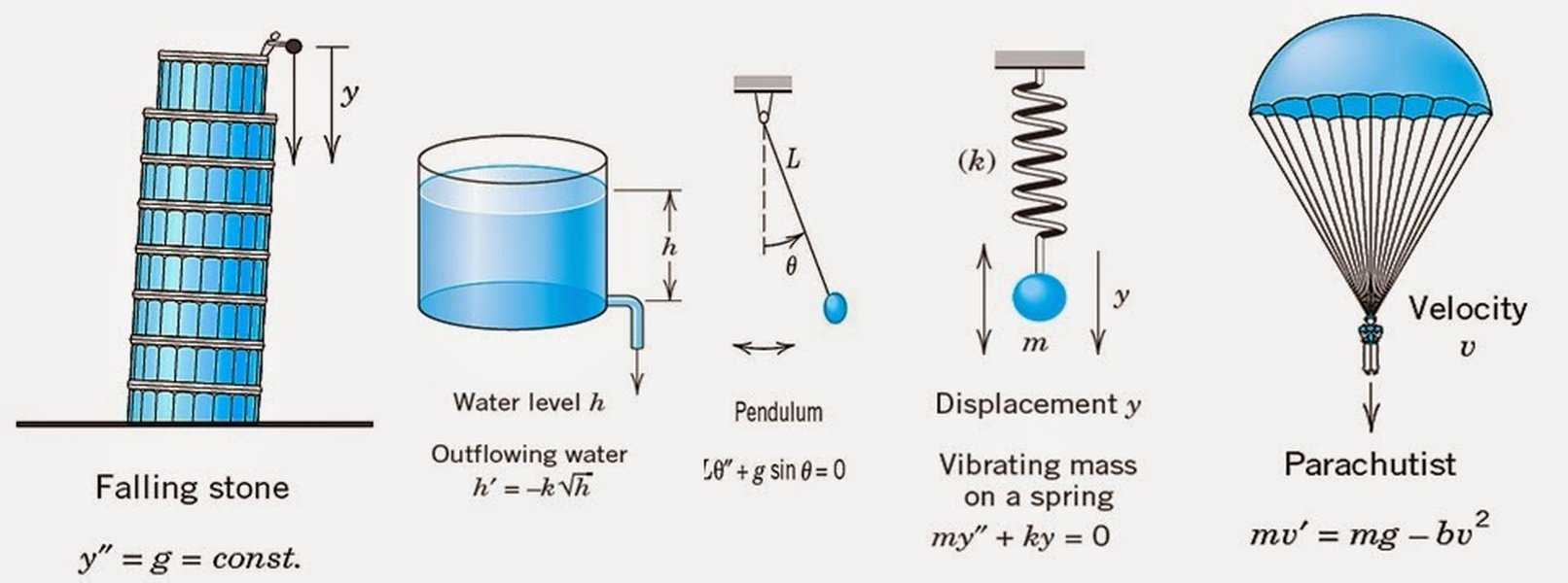
Mechanical Systems: Motion and Vibrations

Newton's second law, \( F = ma \), is inherently a differential equation, as acceleration \( a \) is the second derivative of position with respect to time (\( a = \frac{d^2x}{dt^2} \)). This forms the basis for modeling:

Projectile motion: Describing the path of an object under gravity, possibly with air resistance.
Pendulums: The motion of a simple pendulum is governed by a second-order ODE.
Mass-spring-damper systems: These are classic examples of second-order ODEs used to model vibrations in structures and mechanical devices. The equation is often \( m\frac{d^2x}{dt^2} + c\frac{dx}{dt} + kx = F(t) \).

Electrical Circuits

The behavior of electrical circuits containing resistors (R), inductors (L), and capacitors (C) is described by ODEs derived from Kirchhoff's laws. For an RLC circuit, the equation for the charge \( q \) on the capacitor can be a second-order linear ODE: \( L\frac{d^2q}{dt^2} + R\frac{dq}{dt} + \frac{1}{C}q = V(t) \), where \( V(t) \) is the voltage source. These models are essential for designing and analyzing all electronic devices.

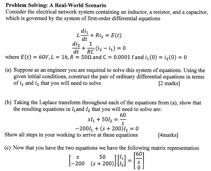
An RLC circuit, whose behavior (current and charge) over time is modeled by ODEs.

Economics and Finance

Economic Growth Models

ODEs are used to model how economies grow over time. The Solow-Swan model, for example, uses a differential equation to describe the evolution of capital per effective worker. These models help economists understand the factors driving long-run economic growth and the impact of policies.

Market Dynamics and Asset Pricing

While often modeled with stochastic differential equations, certain aspects of market behavior or specific deterministic financial models can utilize ODEs, for example, in modeling interest rate dynamics or the growth of investments under continuous compounding (\( \frac{dA}{dt} = rA \)).

Chemistry

Chemical Reaction Kinetics

The rate at which chemical reactions occur is described by ODEs. For a simple reaction \( A \rightarrow B \), the rate of change of the concentration of reactant \( A \), denoted \( [A] \), might be \( \frac{d[A]}{dt} = -k[A]^n \), where \( k \) is the rate constant and \( n \) is the order of the reaction. Systems of ODEs are used for more complex reaction networks.

Mixing Problems

ODEs can model the concentration of a solute in a tank where a solution is entering and leaving. By setting up a balance equation for the rate of change of the amount of solute, one can determine the concentration at any time.

Comparative Impact of ODE Modeling Factors

The success and applicability of an ODE model in solving real-life problems depend on various factors. The radar chart below provides an opinionated comparison of different hypothetical ODE modeling scenarios based on key characteristics. These characteristics influence how well a model can represent reality and how practical it is to implement. The scores are on a scale of 1 (low/poor) to 10 (high/excellent).

This chart visualizes the trade-offs: for example, a complex climate model might have high predictive power and accuracy but also high computational cost and data requirements, with moderate interpretability. In contrast, a simple logistic growth model is highly interpretable and less computationally demanding but might lack accuracy for complex ecological systems. Choosing or developing an ODE model often involves balancing these factors based on the specific problem and available resources.

Key ODE Models and Their Real-World Significance

Certain ODEs appear frequently due to their ability to model fundamental processes. The table below summarizes some common ODE models, their general mathematical form or key concept, and their primary areas of application.

Model Name / Type	General ODE Form / Key Concept	Primary Applications
Exponential Growth/Decay	\( \frac{dP}{dt} = kP \)	Population dynamics (unrestricted), radioactive decay, compound interest, simple chemical reactions.
Logistic Growth	\( \frac{dP}{dt} = rP\left(1 - \frac{P}{K}\right) \)	Population growth with limiting factors (carrying capacity K), spread of rumors or technologies, resource management.
Newton's Law of Cooling/Heating	\( \frac{dT}{dt} = -k(T - T_{\text{env}}) \)	Forensics (time of death), food processing and safety, thermal engineering, material science.
Simple Harmonic Motion (Undamped)	\( m\frac{d^2x}{dt^2} + kx = 0 \) or \( \frac{d^2x}{dt^2} + \omega_0^2 x = 0 \)	Idealized pendulums (small angles), mass-spring systems without friction, basis for AC circuit analysis (analogous equations).
Damped Harmonic Motion	\( m\frac{d^2x}{dt^2} + c\frac{dx}{dt} + kx = 0 \)	Realistic mechanical vibrations (e.g., shock absorbers), RLC circuits, oscillations in physical systems with energy dissipation.
First-Order Linear ODE (General)	\( \frac{dy}{dt} + p(t)y = q(t) \)	Mixing problems, L-R or R-C electrical circuits, decay with continuous input, some financial models. Solved using an integrating factor.
Lotka-Volterra Equations (Predator-Prey)	System of two coupled nonlinear ODEs: \( \frac{dx}{dt} = \alpha x - \beta xy \) (prey) \( \frac{dy}{dt} = \delta xy - \gamma y \) (predator)	Ecology (predator-prey dynamics), epidemiology (some disease models), modeling competitive interactions.
SIR Model (Epidemiology)	System of three coupled ODEs for Susceptible (S), Infected (I), Recovered (R) populations.	Modeling the spread of infectious diseases, predicting epidemic peaks, evaluating public health interventions.

Understanding these fundamental models provides a strong foundation for tackling more complex real-world problems that can often be broken down into, or approximated by, these core types.

Exploring ODE Applications: A Visual Guide

To further illustrate the breadth and importance of differential equations, the following video provides an excellent introduction to what they are, showcases various examples, and touches upon their wide-ranging applications in understanding the world around us. It helps bridge the gap between the mathematical formalism and the tangible phenomena they describe.

This video, "What is a differential equation? Applications and examples," effectively explains that differential equations are equations involving functions and their derivatives. It highlights how they arise naturally when describing change, making them indispensable tools in physics (e.g., motion of objects, wave propagation), biology (e.g., population growth, disease spread), engineering (e.g., circuit analysis, fluid dynamics), and economics (e.g., modeling market trends). By showing concrete examples, it reinforces the idea that ODEs are not just theoretical exercises but powerful instruments for practical problem-solving and prediction.

References

lupucezar.wordpress.com
Last updated May 7, 2025