Understanding Variational Autoencoder (VAE) Theory

A Deep Dive into the Mechanics and Applications of VAEs

Key Takeaways

• Probabilistic Framework: VAEs utilize probabilistic methods to map data into a latent space, enabling the generation of diverse and realistic samples.
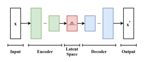
• Encoder-Decoder Architecture: The VAE consists of an encoder that compresses data into a latent distribution and a decoder that reconstructs data from this distribution.
• Effective Training Mechanism: VAEs are trained by optimizing the Evidence Lower Bound (ELBO), which balances reconstruction accuracy and latent space regularization.

---

Introduction to Variational Autoencoders

Variational Autoencoders (VAEs) represent a significant advancement in the field of generative models, merging concepts from deep learning and Bayesian inference. Unlike traditional autoencoders, which encode data into a fixed latent space, VAEs map inputs to probabilistic distributions, allowing for the generation of new, diverse data samples that closely resemble the original dataset.

Core Components of VAEs

Encoder

The encoder in a VAE is a neural network that transforms input data into parameters of a probability distribution in the latent space. Specifically, for each input, the encoder outputs a mean (μ) and a variance (σ²), typically modeling the latent variables as Gaussian distributions. This probabilistic encoding allows the VAE to capture the inherent variability in the data.

Latent Space

The latent space is a lower-dimensional representation of the input data, capturing the essential features in a compressed form. In VAEs, this space is probabilistic, meaning each input corresponds to a distribution rather than a single point. This probabilistic nature facilitates the generation of new data by sampling from the latent distributions.

Sampling

Sampling involves drawing latent variables from the distribution defined by the encoder's output (μ and σ²). To ensure differentiability during training, VAEs employ the "reparameterization trick," where the sampling process is expressed as: $$ z = \mu(x) + \sigma(x) \cdot \epsilon \quad \text{where } \epsilon \sim \mathcal{N}(0, 1) $$ This approach allows gradients to pass through the stochastic sampling step, enabling effective optimization of the model parameters.

Decoder

The decoder is another neural network that maps sampled latent variables back to the original data space. Its primary function is to reconstruct the input data from the latent representation, effectively learning to generate data that mirrors the structure and distribution of the training dataset.

Loss Function: Evidence Lower Bound (ELBO)

The training objective of a VAE is to maximize the Evidence Lower Bound (ELBO), which serves as a proxy for the log-likelihood of the data. The ELBO comprises two main components:

• Reconstruction Loss: Measures the fidelity of the decoder's reconstruction of the input data. Commonly, this is calculated using mean squared error (MSE) or binary cross-entropy.
• Kullback-Leibler (KL) Divergence: Quantifies the difference between the encoder's learned latent distribution and a predefined prior distribution (usually a standard normal distribution). This term enforces regularization, ensuring that the latent space remains structured and supports smooth interpolation.

The ELBO can be mathematically expressed as:

$$ \text{ELBO} = \mathbb{E}_{q(z|x)}[\log p(x|z)] - \text{KL}(q(z|x) \| p(z)) $$

Training Process of VAEs

Training a VAE involves optimizing the ELBO to achieve a balance between accurate data reconstruction and a well-structured latent space. The process can be broken down into the following steps:

1. Forward Pass: An input data point is passed through the encoder to obtain the mean and variance of the latent distribution. A latent variable is then sampled using the reparameterization trick.
2. Reconstruction: The sampled latent variable is fed into the decoder to reconstruct the original data.
3. Loss Computation: The reconstruction loss and KL divergence are calculated.
4. Backpropagation: Gradients of the loss with respect to the model parameters are computed and used to update the weights of both the encoder and decoder networks.

Generative Capabilities of VAEs

Once trained, VAEs can generate new data samples by sampling latent variables from the prior distribution and passing them through the decoder. This generative ability is a result of the model learning the underlying distribution of the training data, allowing it to produce novel yet realistic samples.

Mathematical Foundation of VAEs

VAEs are grounded in variational Bayesian inference, a technique for approximating complex probability distributions. The central idea is to approximate the true posterior distribution of the latent variables given the data, which is often intractable. By introducing a variational distribution (parameterized by the encoder), VAEs can efficiently approximate the posterior and perform effective inference.

The optimization of the ELBO ensures that the variational distribution is as close as possible to the true posterior while maintaining a simple and computationally manageable form.

Advantages of Variational Autoencoders

• Generative Diversity: The probabilistic nature of VAEs allows for the generation of a wide variety of samples, capturing the diversity of the training data.
• Structured Latent Space: The KL divergence term enforces a smooth and continuous latent space, facilitating meaningful interpolations between data points.
• Scalability: VAEs can handle high-dimensional data efficiently, making them suitable for complex tasks like image and text generation.
• Robustness to Noise: The probabilistic framework makes VAEs resilient to noise in the input data, enhancing their performance in real-world applications.

Limitations of VAEs

• Blurry Reconstructions: VAEs may produce less sharp reconstructions, especially in high-dimensional data like images, due to the use of simplistic likelihood models.
• Mode Collapse: VAEs might struggle to capture all modes of a complex dataset, leading to less diverse generated samples compared to models like Generative Adversarial Networks (GANs).
• Computational Complexity: The need to optimize both reconstruction loss and KL divergence can make training VAEs computationally intensive.
• Assumption of Gaussian Latent Space: The common assumption of a Gaussian prior in the latent space may not be suitable for all types of data, limiting the model's flexibility.

Applications of VAEs

• Image Generation: VAEs are employed to create new images that resemble the training dataset, such as generating realistic human faces or artistic creations.
• Anomaly Detection: By learning the distribution of normal data, VAEs can identify outliers or anomalies that do not conform to the learned patterns.
• Data Compression: VAEs effectively compress high-dimensional data into lower-dimensional representations, facilitating efficient storage and transmission.
• Text and Speech Generation: VAEs can generate meaningful text sequences or synthetic speech, contributing to advancements in natural language processing and speech synthesis.
• Reinforcement Learning: In reinforcement learning, VAEs help in learning compact representations of environments, which can enhance the efficiency and effectiveness of learning algorithms.

Enhanced VAE Architectures

Conditional VAEs (CVAEs)

Conditional VAEs extend the VAE framework by introducing additional information as input to both the encoder and decoder. This allows the model to generate data conditioned on specific attributes, enabling controlled data generation.

Deep VAEs

Deep VAEs incorporate multiple layers in both the encoder and decoder networks, enhancing the model's capacity to capture intricate patterns in complex datasets.

Beta-VAE

Beta-VAEs introduce a hyperparameter (β) that scales the KL divergence term in the loss function, promoting disentangled latent representations. This results in more interpretable and separated latent factors.

Implementing a VAE: A Practical Example

Python Implementation with TensorFlow

Below is a simplified example of how a VAE can be implemented using TensorFlow:

import tensorflow as tf
from tensorflow.keras import layers

# Encoder
latent_dim = 2

encoder_inputs = tf.keras.Input(shape=(28, 28, 1))
x = layers.Conv2D(32, 3, activation='relu', strides=2, padding='same')(encoder_inputs)
x = layers.Conv2D(64, 3, activation='relu', strides=2, padding='same')(x)
x = layers.Flatten()(x)
x = layers.Dense(16, activation='relu')(x)
z_mean = layers.Dense(latent_dim, name='z_mean')(x)
z_log_var = layers.Dense(latent_dim, name='z_log_var')(x)

# Sampling layer
def sampling(args):
    z_mean, z_log_var = args
    epsilon = tf.random.normal(shape=(tf.shape(z_mean)[0], latent_dim))
    return z_mean + tf.exp(0.5 * z_log_var) * epsilon

z = layers.Lambda(sampling, output_shape=(latent_dim,), name='z')([z_mean, z_log_var])

# Decoder
decoder_inputs = tf.keras.Input(shape=(latent_dim,))
x = layers.Dense(7 * 7 * 64, activation='relu')(decoder_inputs)
x = layers.Reshape((7, 7, 64))(x)
x = layers.Conv2DTranspose(64, 3, activation='relu', strides=2, padding='same')(x)
x = layers.Conv2DTranspose(32, 3, activation='relu', strides=2, padding='same')(x)
decoder_outputs = layers.Conv2DTranspose(1, 3, activation='sigmoid', padding='same')(x)

# Model
encoder = tf.keras.Model(encoder_inputs, [z_mean, z_log_var, z], name='encoder')
decoder = tf.keras.Model(decoder_inputs, decoder_outputs, name='decoder')
vae_outputs = decoder(encoder(encoder_inputs)[2])
vae = tf.keras.Model(encoder_inputs, vae_outputs, name='vae')

# Loss
reconstruction_loss = tf.keras.losses.binary_crossentropy(tf.keras.backend.flatten(encoder_inputs), tf.keras.backend.flatten(vae_outputs))
reconstruction_loss *= 28 * 28
kl_loss = 1 + z_log_var - tf.square(z_mean) - tf.exp(z_log_var)
kl_loss = tf.reduce_sum(kl_loss, axis=-1)
kl_loss *= -0.5
vae_loss = tf.reduce_mean(reconstruction_loss + kl_loss)
vae.add_loss(vae_loss)
vae.compile(optimizer='adam')
  

Visualizing the VAE Process

The VAE process can be visualized through the following stages:

Stage	Description
Encoding	The input data is passed through the encoder to obtain the latent distribution parameters (μ and σ²).
Sampling	A latent variable is sampled from the distribution using the reparameterization trick.
Decoding	The sampled latent variable is fed into the decoder to reconstruct the original data.
Optimization	The ELBO loss is computed and optimized to improve both reconstruction and latent space structure.

---

Advanced Topics in VAE Theory

Disentangled Representations

Disentanglement refers to the ability of the VAE to learn latent factors that are independent and interpretable. Methods like Beta-VAE introduce additional constraints to promote disentanglement, enabling the model to capture distinct generative factors in separate dimensions of the latent space.

Hierarchical VAEs

Hierarchical VAEs incorporate multiple layers of latent variables, allowing the model to capture complex dependencies and hierarchical structures in the data. This enhances the model's capacity to generate more intricate and high-fidelity samples.

Semi-Supervised VAEs

In semi-supervised settings, VAEs can leverage both labeled and unlabeled data to improve learning. By conditioning the latent space on label information, the model can achieve better generalization and interpretability.

Practical Considerations

Choosing the Latent Dimension

Selecting the appropriate dimensionality for the latent space is crucial. A smaller latent dimension enforces more compression but may lead to loss of important information, while a larger dimension may capture more details but risk overfitting and less meaningful representations.

Balancing the ELBO Components

The balance between reconstruction loss and KL divergence is essential for effective training. Techniques such as annealing the KL term or adjusting the beta parameter in Beta-VAEs can help achieve a better trade-off between data fidelity and latent space regularization.

Regularization Techniques

Regularization strategies, such as dropout or weight decay, can be employed to prevent overfitting and improve the generalization capabilities of the VAE.

Conclusion

Variational Autoencoders stand as a powerful framework for generative modeling, offering a blend of deep learning and probabilistic reasoning. Their ability to learn meaningful latent representations and generate diverse data samples makes them invaluable in various applications, from image synthesis to anomaly detection. While they come with certain limitations, ongoing research and advancements continue to enhance their capabilities and extend their applicability.

References

Last updated January 19, 2025