
Unlocking the Secrets of Magnetism: A Deep Dive for AP Physics C E&M
From foundational laws and calculus-based equations to intuitive understanding and real-world applications.
Welcome to an in-depth exploration of magnetism as covered in the AP Physics C: Electricity and Magnetism (E&M) curriculum. This calculus-based journey will take you through the fundamental principles governing magnetic fields, the forces they exert, how they are generated, and their intimate connection with electricity, all framed by Maxwell's unifying equations.
Essential Insights into Magnetism
- Moving Charges are Key: Unlike static electric fields generated by charges, magnetic fields originate from moving electric charges (currents) or the intrinsic magnetic moments of elementary particles.
- Forces and Fields Interplay: Magnetic fields exert forces on other moving charges and current-carrying conductors, but this force is always perpendicular to both the velocity and the field, meaning magnetic fields alone do no work on charges.
- Electricity and Magnetism are Unified: Maxwell's equations reveal that electricity and magnetism are two facets of the same fundamental force (electromagnetism), where changing electric fields create magnetic fields, and changing magnetic fields induce electric fields (electromagnetic induction).
The Nature of Magnetic Fields
What is a Magnetic Field?
A magnetic field, denoted by the vector \(\vec{B}\), is a region of space where magnetic influence can be detected. It exerts forces on moving electric charges and magnetic materials. The SI unit for magnetic field strength is the Tesla (T).
Magnetic fields are visualized using magnetic field lines. Unlike electric field lines that originate and terminate on charges, magnetic field lines always form closed loops. This is a fundamental difference and points to the absence of magnetic monopoles (isolated north or south poles) in nature.
Gauss's Law for Magnetism
This concept is mathematically expressed by Gauss's Law for Magnetism, one of Maxwell's equations:
\[ \nabla \cdot \vec{B} = 0 \]Or in integral form, stating that the net magnetic flux through any closed surface is zero:
\[ \oint_S \vec{B} \cdot d\vec{A} = 0 \]This mathematically confirms that magnetic field lines are continuous loops with no starting or ending points.
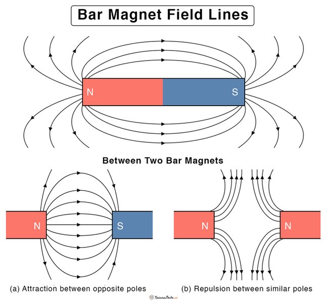
Visual representation of magnetic field lines forming closed loops around a bar magnet.
Forces Exerted by Magnetic Fields
The Lorentz Force Law
The fundamental interaction between a magnetic field and a moving charge is described by the magnetic part of the Lorentz force. The total Lorentz force includes both electric (\(\vec{E}\)) and magnetic (\(\vec{B}\)) fields acting on a charge \(q\) moving with velocity \(\vec{v}\):
\[ \vec{F} = q(\vec{E} + \vec{v} \times \vec{B}) \]Focusing on the magnetic component:
\[ \vec{F}_B = q(\vec{v} \times \vec{B}) \]Key Characteristics of the Magnetic Force:
- Direction: The force \(\vec{F}_B\) is always perpendicular to both the velocity \(\vec{v}\) and the magnetic field \(\vec{B}\). Its direction can be determined using the right-hand rule (for positive charges).
- Magnitude: The magnitude of the force is given by \(F_B = |q|vB\sin\theta\), where \(\theta\) is the angle between \(\vec{v}\) and \(\vec{B}\).
- Zero Force Conditions: The magnetic force is zero if the charge is stationary (\(v=0\)) or if the velocity is parallel or anti-parallel to the magnetic field (\(\theta = 0^\circ\) or \(\theta = 180^\circ\)).
- Work: Since the magnetic force is always perpendicular to the direction of motion (velocity), it does no work on the charged particle (\(W = \int \vec{F}_B \cdot d\vec{l} = 0\)). It can change the direction of motion but not the kinetic energy or speed of the particle.
Force on a Current-Carrying Wire
A wire carrying a current \(I\) consists of moving charges. Therefore, a segment of wire of length \(L\) placed in a magnetic field \(\vec{B}\) experiences a magnetic force. For a straight wire segment represented by vector \(\vec{L}\) (pointing in the direction of current), the force is:
\[ \vec{F}_B = I(\vec{L} \times \vec{B}) \]The direction is again found using the right-hand rule. This principle is fundamental to the operation of electric motors.
Sources of Magnetic Fields
Magnetic fields are generated by moving electric charges, either as individual particles or collectively as an electric current.
The Biot-Savart Law
The Biot-Savart Law allows for the calculation of the magnetic field produced by a steady current distribution. It gives the differential magnetic field \(d\vec{B}\) produced at a point by an infinitesimal current element \(I d\vec{l}\):
\[ d\vec{B} = \frac{\mu_0}{4\pi} \frac{I d\vec{l} \times \hat{r}}{r^2} \] Where:- \(\mu_0\) is the permeability of free space (\(4\pi \times 10^{-7} \, \text{T}\cdot\text{m/A}\)).
- \(I\) is the current.
- \(d\vec{l}\) is an infinitesimal vector element of the wire pointing in the direction of the current.
- \(\hat{r}\) is the unit vector pointing from the current element \(d\vec{l}\) to the point where the field is being calculated.
- \(r\) is the distance from the current element to the point.
To find the total magnetic field \(\vec{B}\) from a complete circuit or wire configuration, one must integrate these contributions over the entire current path. This often requires vector calculus.
Example: Field of a Long Straight Wire
Using the Biot-Savart Law (or Ampère's Law, see below), the magnitude of the magnetic field at a perpendicular distance \(r\) from a long, straight wire carrying current \(I\) is:
\[ B = \frac{\mu_0 I}{2\pi r} \]The magnetic field lines form concentric circles around the wire, with the direction given by the right-hand rule (thumb along current, fingers curl in field direction).
Ampère's Law
Ampère's Law provides an alternative, often simpler, way to calculate magnetic fields, especially in situations with high symmetry (like long wires, solenoids, toroids). In its original form, it relates the line integral of the magnetic field around a closed loop (an "Amperian loop") to the total steady current \(I_{enc}\) passing through the surface enclosed by the loop:
\[ \oint \vec{B} \cdot d\vec{l} = \mu_0 I_{enc} \]Example: Field Inside a Long Solenoid
A solenoid is a coil wound into a tightly packed helix. For an ideal, long solenoid with \(n\) turns per unit length carrying current \(I\), Ampère's Law yields a uniform magnetic field inside:
\[ B = \mu_0 n I \]The field outside is ideally zero.
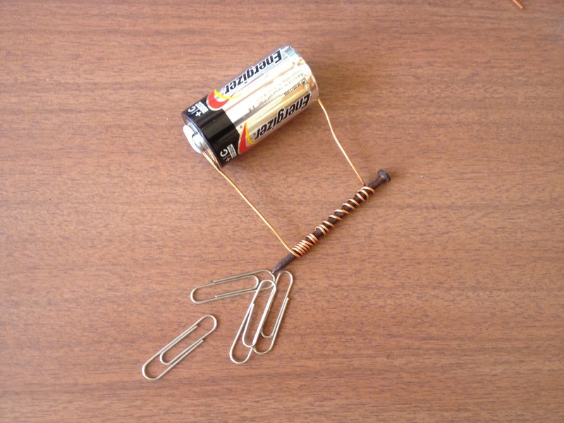
A simple electromagnet, demonstrating how current in a coil (solenoid) creates a magnetic field.
Maxwell's Equations and the Unification
James Clerk Maxwell unified electricity and magnetism into a single theory of electromagnetism, described by four fundamental equations. Two are Gauss's laws (for E and B fields), and the other two connect changing fields.
Faraday's Law of Induction
Faraday discovered that a changing magnetic flux through a loop induces an electromotive force (emf), and thus can drive a current. This is electromagnetic induction, the principle behind electric generators and transformers.
Mathematically, Faraday's Law (Maxwell's third equation) relates the induced electric field \(\vec{E}\) to the changing magnetic field \(\vec{B}\):
\[ \nabla \times \vec{E} = - \frac{\partial \vec{B}}{\partial t} \]The integral form gives the induced emf (\(\mathcal{E}\)) around a closed loop:
\[ \mathcal{E} = \oint \vec{E} \cdot d\vec{l} = -\frac{d\Phi_B}{dt} \] Where \(\Phi_B = \int \vec{B} \cdot d\vec{A}\) is the magnetic flux through the loop. The negative sign (Lenz's Law) indicates that the induced current creates a magnetic field opposing the change in flux.Ampère-Maxwell Law
Maxwell realized Ampère's original law was incomplete for situations involving changing electric fields (like charging capacitors). He added a crucial term, the "displacement current," proportional to the rate of change of electric flux (\(\frac{\partial \vec{E}}{\partial t}\)). The complete Ampère-Maxwell Law (Maxwell's fourth equation) is:
\[ \nabla \times \vec{B} = \mu_0 \vec{J} + \mu_0 \epsilon_0 \frac{\partial \vec{E}}{\partial t} \] Where \(\vec{J}\) is the conduction current density and \(\epsilon_0\) is the permittivity of free space. The integral form is: \[ \oint \vec{B} \cdot d\vec{l} = \mu_0 I_{enc} + \mu_0 \epsilon_0 \frac{d\Phi_E}{dt} \]This equation shows that magnetic fields are produced not only by currents (\(\mu_0 \vec{J}\)) but also by changing electric fields (\(\mu_0 \epsilon_0 \frac{\partial \vec{E}}{\partial t}\)). This term completed the symmetry between electricity and magnetism and was essential for predicting the existence of electromagnetic waves (light).
Key Concepts and Equations Summary Table
This table summarizes the core equations and concepts discussed, crucial for AP Physics C E&M:
| Concept | Equation (Vector Form) | Description | Key Variables |
|---|---|---|---|
| Magnetic Force (Lorentz) | \(\vec{F}_B = q(\vec{v} \times \vec{B})\) | Force on a moving charge in a B-field. | \(q\): charge, \(\vec{v}\): velocity, \(\vec{B}\): magnetic field |
| Force on Current Wire | \(\vec{F}_B = I(\vec{L} \times \vec{B})\) | Force on a current-carrying wire segment in a B-field. | \(I\): current, \(\vec{L}\): length vector, \(\vec{B}\): magnetic field |
| Biot-Savart Law | \(d\vec{B} = \frac{\mu_0}{4\pi} \frac{I d\vec{l} \times \hat{r}}{r^2}\) | Calculates B-field from a differential current element. | \(\mu_0\): permeability, \(I\): current, \(d\vec{l}\): wire element, \(\hat{r}\): unit vector, \(r\): distance |
| Ampère's Law (Original) | \(\oint \vec{B} \cdot d\vec{l} = \mu_0 I_{enc}\) | Relates B-field circulation to enclosed steady current. | \(\vec{B}\): magnetic field, \(d\vec{l}\): path element, \(I_{enc}\): enclosed current |
| Gauss's Law for Magnetism | \(\oint_S \vec{B} \cdot d\vec{A} = 0\) | States net magnetic flux through a closed surface is zero (no monopoles). | \(\vec{B}\): magnetic field, \(d\vec{A}\): area element |
| Faraday's Law | \(\oint \vec{E} \cdot d\vec{l} = -\frac{d\Phi_B}{dt}\) | Changing magnetic flux induces an emf (electric field). | \(\vec{E}\): electric field, \(\Phi_B\): magnetic flux, \(t\): time |
| Ampère-Maxwell Law | \(\oint \vec{B} \cdot d\vec{l} = \mu_0 I_{enc} + \mu_0 \epsilon_0 \frac{d\Phi_E}{dt}\) | Relates B-field circulation to enclosed current AND changing electric flux. | \(I_{enc}\): current, \(\epsilon_0\): permittivity, \(\Phi_E\): electric flux |
Developing Intuition for Magnetism
Building physical intuition alongside mathematical formalism is vital:
- Right-Hand Rules: Master the various right-hand rules to quickly determine directions of fields (around wires), forces (Lorentz), and induced currents (Lenz's Law).
- Field Lines Visualization: Always picture magnetic field lines as closed loops. Where lines are denser, the field is stronger.
- Force Perpendicularity: Remember the magnetic force is always perpendicular to \(\vec{v}\) and \(\vec{B}\). This leads to circular or helical motion for charges in uniform fields and explains why magnetic fields don't change a particle's speed.
- Source-Field Relationship: Currents create circulating magnetic fields around them. Think of the field wrapping around the current source.
- Induction as a Response: Lenz's Law (the minus sign in Faraday's Law) reflects nature's tendency to oppose change. An induced current flows in a direction to create a magnetic field that counteracts the *change* in magnetic flux.
- Relativistic Connection (Conceptual): While not explicitly derived in AP Physics C, understanding that magnetism can be viewed as a relativistic consequence of electricity provides deeper insight. What one observer sees as an electric field, a moving observer might perceive as a combination of electric and magnetic fields.
Conceptual Overview: Magnetism Mindmap
This mindmap provides a visual structure connecting the core concepts of magnetism covered in AP Physics C E&M, showing their relationships and hierarchy.
∇ · B = 0"] id2["Magnetic Forces"] id2a["Lorentz Force"] id2a1["On Moving Charge
F = q(v x B)"] id2a2["Perpendicular to v and B"] id2a3["Does No Work"] id2a4["Right-Hand Rule"] id2b["On Current-Carrying Wire"] id2b1["F = I(L x B)"] id2b2["Basis for Motors"] id2c["Between Parallel Wires"] id2c1["Attraction (Parallel Currents)"] id2c2["Repulsion (Anti-parallel Currents)"] id3["Calculating Magnetic Fields"] id3a["Biot-Savart Law"] id3a1["dB = (μ₀/4π) (I dl x r̂) / r²"] id3a2["Integration over Current Distribution"] id3a3["Requires Calculus"] id3b["Ampère's Law"] id3b1["∮ B · dl = μ₀ I_enc"] id3b2["Useful for Symmetric Cases
(Wire, Solenoid, Toroid)"] id3b3["Requires Calculus (Line Integral)"] id4["Electromagnetism & Maxwell's Eq."] id4a["Faraday's Law of Induction"] id4a1["∇ x E = -∂B/∂t"] id4a2["∮ E · dl = -dΦ_B/dt"] id4a3["Changing B creates E"] id4a4["Lenz's Law (Opposes Change)"] id4b["Ampère-Maxwell Law"] id4b1["∇ x B = μ₀J + μ₀ε₀ ∂E/∂t"] id4b2["∮ B · dl = μ₀I_enc + μ₀ε₀ dΦ_E/dt"] id4b3["Currents & Changing E create B"] id4b4["Displacement Current"] id4c["Unification of E & M"] id4d["Prediction of EM Waves"] id5["Applications & Examples"] id5a["Long Straight Wire Field"] id5b["Solenoid / Toroid Field"] id5c["Force Between Wires"] id5d["Torque on Current Loop"] id5d1["Magnetic Dipole Moment (μ = IA)"] id5d2["τ = μ x B"] id5e["Electric Motors"] id5f["Generators"] id5g["Mass Spectrometers"] id5h["Particle Accelerators"]
Comparative Analysis of Magnetism Concepts
This chart offers a relative comparison of key magnetism concepts encountered in AP Physics C E&M based on typical student experience regarding difficulty, importance for the exam, conceptual depth, required calculus intensity, and range of applications.
Video Review: Magnetic Fields Basics
For a visual and auditory review of the fundamentals of magnetic fields, including dipoles and basic interactions relevant to AP Physics C E&M, consider this helpful video:
This video covers the basics of magnetic dipoles, ferromagnetic and paramagnetic materials, and introduces concepts essential for understanding magnetic fields in the AP Physics C E&M course.
Frequently Asked Questions (FAQ)
► Why are there no magnetic monopoles?
► Why doesn't the magnetic force do work on a charged particle?
► When should I use Biot-Savart vs. Ampère's Law?
► What is the significance of Maxwell's displacement current?
Recommended Further Exploration
- How can you calculate the magnetic field inside and outside a coaxial cable using Ampere's Law?
- What is the step-by-step derivation for the torque on a rectangular current loop in a uniform magnetic field?
- How does a velocity selector use combined electric and magnetic fields to filter charged particles by speed?
- What is the magnetic vector potential and how does it relate to the magnetic field?
References
Last updated May 5, 2025