Solving Gauss's Law for a Point Charge: Formula and Python Implementation

Introduction to Maxwell's Equations

Maxwell's equations are the cornerstone of classical electromagnetism, encapsulating the behavior of electric and magnetic fields and their interactions with matter. These four equations—Gauss's Law for Electricity, Gauss's Law for Magnetism, Faraday's Law of Induction, and Ampère-Maxwell Law—are interrelated and collectively describe how electric and magnetic fields propagate and interact. However, each equation holds significant importance on its own, allowing us to solve specific electromagnetic problems under certain conditions.

In this comprehensive guide, we will focus on one of Maxwell's equations: Gauss's Law for Electricity. We will delve into its formulation, explore its application in calculating the electric field around a point charge, and provide a simple Python implementation to visualize the results.

Gauss's Law for Electricity

Mathematical Formulation

Gauss's Law relates the distribution of electric charge to the resulting electric field. It is fundamental in determining electric fields around symmetric charge distributions. Gauss's Law can be expressed in two forms: the integral form and the differential form.

Integral Form

The integral form of Gauss's Law is given by:

∮ E ⋅ dA = Q / ε₀

Where:

• ∮ E ⋅ dA: The closed surface integral of the electric field E over a closed surface A. This represents the total electric flux through the surface.
• Q: The total electric charge enclosed within the surface.
• ε₀: The vacuum permittivity or electric constant, approximately 8.854187817 × 10-12 F/m.

Differential Form

The differential form of Gauss's Law is expressed as:

∇ ⋅ E = ρ / ε₀

Where:

• ∇ ⋅ E: The divergence of the electric field, representing the net flux out of an infinitesimal volume.
• ρ: The volume charge density, or charge per unit volume.

Application: Electric Field of a Point Charge

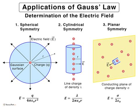
One of the most straightforward applications of Gauss's Law is determining the electric field generated by a point charge. This scenario leverages the spherical symmetry of the charge distribution, making the integral form of Gauss's Law particularly convenient.

Deriving the Electric Field

Consider a point charge q located at the origin. To find the electric field at a distance r from the charge, we follow these steps:

1. Select a Gaussian Surface: Choose a spherical surface of radius r centered at the point charge. The symmetry ensures that the electric field has the same magnitude at every point on the surface and points radially outward.
2. Apply Gauss's Law: Substitute the chosen Gaussian surface into the integral form of Gauss's Law.
3. Simplify the Equation: Due to symmetry, the electric field E is constant in magnitude over the surface and perpendicular to it, allowing us to take E out of the integral.
4. Solve for E: Rearrange the equation to solve for the electric field.

Following these steps, the electric field due to a point charge is derived as:

E = ^q/(4πε₀r²)

This equation is also known as Coulomb's Law, which quantifies the electric field generated by a stationary point charge.

Python Implementation

To visualize the electric field around a point charge, we can implement a simple Python script. This script will compute the electric field at various distances from the charge and plot the results, demonstrating the inverse square relationship.

Prerequisites

Ensure you have the following Python libraries installed:

• NumPy: For numerical operations.
• Matplotlib: For plotting graphs.

You can install these libraries using pip if they are not already installed:

pip install numpy matplotlib

Code Explanation

1. Importing Libraries: Import the necessary libraries for numerical computations and plotting.
2. Defining Constants: Define the vacuum permittivity ε₀ and Coulomb's constant.
3. Electric Field Function: Create a function to calculate the electric field at a given distance from the point charge.
4. Plotting Function: Develop a function to plot the electric field against distance, showcasing the inverse square law.
5. Main Execution: Execute example calculations and generate the plot.

Complete Python Code

import numpy as np
import matplotlib.pyplot as plt

# Physical constants
EPSILON_0 = 8.854187817e-12  # Permittivity of free space (F/m)
COULOMB_CONSTANT = 1 / (4 * np.pi * EPSILON_0)  # Coulomb's constant (N·m²/C²)

def electric_field_point_charge(charge, distance):
    """
    Calculate the electric field strength at a given distance from a point charge.
    
    Parameters:
        charge (float): The electric charge in Coulombs (C).
        distance (float): The distance from the charge in meters (m).
        
    Returns:
        float: Electric field strength in Newtons per Coulomb (N/C).
    """
    if distance == 0:
        return float('inf')  # Electric field is infinite at the location of the point charge
    else:
        return COULOMB_CONSTANT * charge / (distance ** 2)

def plot_electric_field():
    # Define range of distances from the charge
    distances = np.linspace(0.1, 2, 1000)  # Avoid r=0 to prevent division by zero
    charge = 1e-6  # 1 microCoulomb
    fields = electric_field_point_charge(charge, distances)
    
    # Plotting the electric field vs. distance
    plt.figure(figsize=(10, 6))
    plt.plot(distances, fields, label=f'Electric Field (Q={charge} C)', color='blue')
    plt.title('Electric Field Strength vs. Distance from a Point Charge')
    plt.xlabel('Distance from Charge (m)')
    plt.ylabel('Electric Field Strength (N/C)')
    plt.grid(True)
    plt.yscale('log')  # Logarithmic scale to clearly show the inverse square relationship
    plt.legend()
    plt.show()

if __name__ == "__main__":
    # Example calculations
    test_charge = 1e-6  # 1 microCoulomb
    test_distances = [0.5, 1.0, 1.5, 2.0]  # Distances in meters
    
    print("Electric Field Strength for a 1 µC Charge at Various Distances:")
    print("-" * 50)
    print("{:<15} | {:<20}".format("Distance (m)", "Electric Field (N/C)"))
    print("-" * 50)
    
    for r in test_distances:
        E = electric_field_point_charge(test_charge, r)
        print("{:<15.2f} | {:<20.2e}".format(r, E))
    
    # Demonstrate the inverse square law
    print("\nDemonstrating Inverse Square Law:")
    d1 = 1.0  # Initial distance
    d2 = 2.0  # Double the distance
    f1 = electric_field_point_charge(test_charge, d1)
    f2 = electric_field_point_charge(test_charge, d2)
    print(f"Field at {d1} m: {f1:.2e} N/C")
    print(f"Field at {d2} m: {f2:.2e} N/C")
    print(f"Ratio f1/f2: {f1/f2:.2f} (Should be approximately 4)")
    
    # Plot the electric field
    plot_electric_field()
    

Understanding the Code

1. Importing Libraries:
   • numpy: Utilized for efficient numerical computations, especially for handling arrays of distances and field values.
   • matplotlib.pyplot: Employed for creating plots to visualize the relationship between electric field strength and distance.
2. Defining Physical Constants:
   • EPSILON_0: Represents the vacuum permittivity, a fundamental constant in electromagnetism.
   • COULOMB_CONSTANT: Derived from the vacuum permittivity, it quantifies the electric force between two charges separated by a unit distance.
3. Electric Field Function (electric_field_point_charge):
   • This function calculates the electric field strength at a given distance from a point charge using Coulomb's Law.
   • It handles the singularity at distance = 0 by returning infinity, acknowledging the theoretical infinite field at the exact location of a point charge.
   • The formula implemented is:

     E = (1 / (4πε₀)) * q / r²

4. Plotting Function (plot_electric_field):
   • Generates a range of distances from 0.1 m to 2 m, avoiding r = 0 to prevent division by zero errors.
   • Calculates the electric field at each distance using the previously defined function.
   • Plots the electric field against distance on a logarithmic scale to clearly depict the inverse square relationship.
5. Main Execution Block:
   • Performs example calculations for specific distances, showcasing the electric field values at those points.
   • Demonstrates the inverse square law by comparing electric field values at distances d1 = 1.0 m and d2 = 2.0 m, expecting the field strength at d1 to be four times that at d2.
   • Calls the plotting function to visualize the electric field distribution.

Sample Output

Upon running the script, you will observe the following:

• Console Output: A table displaying the electric field strengths at specified distances and a demonstration of the inverse square law.
• Plot: A graph showing the electric field strength decreasing with the square of the distance from the point charge, visualized on a logarithmic scale for clarity.

Console Output Example:

Electric Field Strength for a 1 µC Charge at Various Distances:
--------------------------------------------------
Distance (m)    | Electric Field (N/C) 
--------------------------------------------------
0.50           | 7.15e+10            
1.00           | 1.79e+10            
1.50           | 7.96e+09            
2.00           | 4.48e+09            

Demonstrating Inverse Square Law:
Field at 1.0 m: 1.79e+10 N/C
Field at 2.0 m: 4.48e+09 N/C
Ratio f1/f2: 4.00 (Should be approximately 4)
    

Plot: The generated plot will display a smooth curve showing the electric field strength decreasing as the distance from the charge increases, adhering to the inverse square law.

Physical Insights

• Inverse Square Law: The electric field strength decreases proportionally to the square of the distance from the point charge. This relationship is clearly depicted in the plot and the demonstration of the inverse square law.
• Singularity at Origin: The electric field theoretically becomes infinite at the exact location of the point charge (r = 0), highlighting the idealization inherent in the concept of a point charge.
• Role of Vacuum Permittivity: The constant ε₀ plays a crucial role in determining the strength of the electric field, encapsulating how electric fields propagate through a vacuum.

Limitations and Considerations

• Point Charge Idealization: Real-world charges are distributed over volumes or surfaces, and the concept of a perfect point charge is an idealization that simplifies calculations.
• Static Conditions: This analysis assumes static charges and fields. In dynamic situations where charges move or fields change with time, other Maxwell's equations become relevant.
• Environmental Factors: The presence of other charges, magnetic fields, or dielectric materials can influence the electric field, necessitating more complex models.

Conclusion

Gauss's Law for Electricity offers a powerful method to calculate electric fields, especially in scenarios with high symmetry, such as point charges or uniformly charged spheres. By leveraging the symmetry of the charge distribution, we can simplify complex problems and derive elegant expressions for electric fields.

The provided Python implementation serves as a practical tool to visualize the inverse square relationship inherent in Coulomb's Law. Through computational simulation, we gain deeper insights into the behavior of electric fields, reinforcing theoretical concepts with empirical visualization.

While Gauss's Law is immensely useful, it's essential to recognize its scope and limitations. In dynamic systems involving time-varying fields or non-symmetric charge distributions, the full suite of Maxwell's equations must be employed to accurately describe electromagnetic phenomena.

Understanding and applying Gauss's Law lays the foundation for exploring more intricate aspects of electromagnetism, paving the way for advancements in physics, engineering, and technology.

References

1. Maxwell's Equations: For a comprehensive overview of Maxwell's equations, refer to the Wikipedia page on Maxwell's Equations.
2. Fundamentals of Physics: For an in-depth exploration of Gauss's Law and its applications, consult standard physics textbooks such as "Fundamentals of Physics" by Halliday, Resnick, and Walker.
3. Python Documentation: For more information on the numpy and matplotlib libraries, visit the NumPy Documentation and the Matplotlib Documentation.
4. Electromagnetism Tutorials: For additional tutorials and examples on electromagnetism and computational simulations, platforms like Khan Academy and Coursera offer valuable resources.