
Unlocking the Power of Quantile Regression: When the Quantile Function Perfectly Minimizes Check Loss
Discover how the foundational mathematics of quantile regression creates robust predictions beyond traditional mean-based approaches
Key Insights on Quantile Function Optimization
- The quantile function minimizes the check loss function precisely when it equals the τ-th conditional quantile of the response variable's distribution
- Check loss creates asymmetric penalties—overestimation and underestimation errors are weighted differently based on the target quantile
- This minimization principle enables quantile regression to model the entire conditional distribution, not just the mean
Understanding the Check Loss Function
The check loss function (also known as pinball loss or quantile loss) is the cornerstone of quantile regression methodology. This specialized loss function enables machine learning models and statistical methods to estimate specific quantiles of a distribution rather than just the central tendency.
Mathematical Definition
The check loss function for a quantile level τ (where 0 ≤ τ ≤ 1) is defined as:
\[ \rho_\tau(u) = \begin{cases} \tau u & \text{if } u \geq 0 \ (\tau - 1)u & \text{if } u < 0 \end{cases} \]Where u represents the residual, defined as the difference between the observed value y and the predicted quantile value ŷ (u = y - ŷ).
This can also be written in a more compact form as:
\[ \rho_\tau(u) = u(\tau - \mathbf{1}\{u < 0\}) \]Where 1{u < 0} is an indicator function that equals 1 when u < 0 and 0 otherwise.
Visual Interpretation
The check loss function creates an asymmetric V-shaped curve where the slopes of the two sides differ based on the quantile level τ:
- For positive residuals (underestimation), the penalty is τ times the residual
- For negative residuals (overestimation), the penalty is (1-τ) times the absolute residual
This asymmetry is the key feature that allows the function to target specific quantiles rather than just the mean or median.
When Does Minimization Occur?
The quantile function minimizes the check loss function under specific mathematical conditions that are fundamental to understanding quantile regression.
Formal Minimization Condition
For a random variable Y and a quantile level τ, the τ-th quantile function qτ(X) minimizes the expected check loss when:
\[ q_\tau(X) = \arg\min_{q} \mathbb{E}[\rho_\tau(Y - q(X))] \]This mathematical formulation states that the quantile function that minimizes the expected check loss is precisely the conditional τ-th quantile of the response variable Y given the predictor variables X.
Proof of Minimization
To understand why this holds true, consider the derivative of the expected check loss with respect to the predicted value q:
\[ \frac{d}{dq} \mathbb{E}[\rho_\tau(Y - q)] = \tau \cdot P(Y \geq q) - (1-\tau) \cdot P(Y < q) \]Setting this derivative to zero and solving:
\[ \tau \cdot P(Y \geq q) = (1-\tau) \cdot P(Y < q) \]Since P(Y ≥ q) = 1 - P(Y < q), we can substitute and solve:
\[ \tau \cdot (1 - P(Y < q)) = (1-\tau) \cdot P(Y < q)\ \tau - \tau \cdot P(Y < q) = (1-\tau) \cdot P(Y < q)\ \tau = P(Y < q) \cdot (1-\tau + \tau)\ \tau = P(Y < q) \]This final equation, τ = P(Y < q), is precisely the definition of the τ-th quantile of Y, confirming that the value q that minimizes the expected check loss is indeed the τ-th quantile.
Special Cases
- When τ = 0.5, the check loss minimization yields the median (as opposed to the mean in squared error minimization)
- When τ = 0.25, the solution corresponds to the first quartile
- When τ = 0.75, the solution corresponds to the third quartile
Visualizing the Minimization Relationship
The following radar chart illustrates how different loss functions compare across various statistical properties, highlighting the unique characteristics of the check loss function that make it ideal for quantile estimation:
The radar chart demonstrates why the check loss function excels in specific areas like robustness to outliers, handling skewed data, and providing accurate uncertainty quantification—all critical for quantile regression applications.
The Conceptual Framework of Quantile Regression
The following mindmap illustrates the key concepts surrounding quantile regression and the check loss function minimization:
Practical Example of Quantile Regression
Let's examine how quantile regression compares to ordinary least squares (OLS) regression in a practical scenario. Consider a dataset where we're modeling the relationship between years of experience (X) and salary (Y):
| Model Type | Objective | Loss Function | Minimization Result | Interpretation |
|---|---|---|---|---|
| OLS Regression | Estimate mean of Y|X | Squared Error: (y - ŷ)² | E[Y|X] | Average salary for given experience |
| Median Regression (τ=0.5) | Estimate median of Y|X | Check Loss: 0.5|y - ŷ| for y≥ŷ, 0.5|y - ŷ| for y<ŷ | Median[Y|X] | Median salary for given experience |
| Q1 Regression (τ=0.25) | Estimate 25th percentile of Y|X | Check Loss: 0.25|y - ŷ| for y≥ŷ, 0.75|y - ŷ| for y<ŷ | Q1[Y|X] | 25th percentile salary for given experience |
| Q3 Regression (τ=0.75) | Estimate 75th percentile of Y|X | Check Loss: 0.75|y - ŷ| for y≥ŷ, 0.25|y - ŷ| for y<ŷ | Q3[Y|X] | 75th percentile salary for given experience |
In this example, quantile regression provides a much more comprehensive view of how salaries vary with experience compared to OLS regression, which only gives the mean relationship.
Visual Demonstration of Check Loss Minimization
For a deeper understanding, watch this video explaining quantile loss and its application in regression models:
This video explains the quantile loss function's structure and how it works to target specific quantiles in statistical modeling—precisely illustrating the minimization principles we've discussed.
Relevant Applications of Quantile Regression
Financial Risk Assessment
In financial risk management, quantile regression is used to estimate Value-at-Risk (VaR) by minimizing the check loss at specific quantiles (typically τ = 0.01 or τ = 0.05). This approach provides more accurate risk estimates than traditional methods, especially in non-normal market conditions.
Environmental Science
Researchers use quantile regression to model the relationship between environmental factors and extreme events. By targeting higher quantiles (e.g., τ = 0.9 or τ = 0.95), scientists can better understand the drivers of extreme temperatures, precipitation levels, or pollution concentrations.
Medical Outcome Prediction
In healthcare analytics, quantile regression helps predict patient outcomes across different risk levels. For instance, estimating recovery times at various quantiles provides a more complete picture than simply predicting the average recovery time.
Economic Growth Analysis
Economists apply quantile regression to understand how various factors affect economic growth differently across developing versus developed nations, or struggling versus thriving sectors.
Illustrative Images

Visual representation of how quantile regression (colored lines) provides estimates at different quantiles of the distribution, compared to OLS regression (black line).
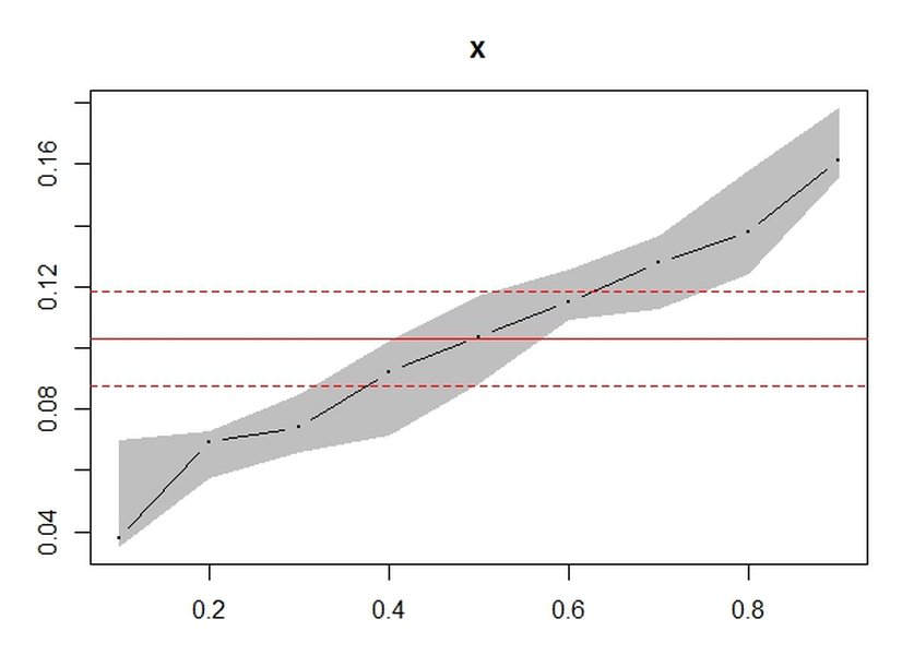
How coefficient estimates can vary across different quantiles, revealing relationships that would be missed by traditional regression methods.
Frequently Asked Questions
References
- Quantile Loss in Neural Networks - Medium
-
Quantile Loss & Quantile Regression - Towards Data Science
- Quantile regression: Loss function - Cross Validated
- Quantile regression - "check function" - Cross Validated
- Quantile regression - Wikipedia
-
Quantile Regression: A Statistical Tool for Out-of-Hospital Research - NCBI
- Efficient Quantile Regression for Heteroscedastic Models - Ohio State University
- Getting Started with Quantile Regression - UVA Library
Recommended Searches
Last updated April 8, 2025