
Understanding Stokes Formula
An in-depth exploration of Stokes’ Law and related concepts
Highlights
- Stokes’ Law and Formula: Describes the drag force acting on small spherical objects in viscous fluids.
- Key Variables: Fluid viscosity, particle radius, and particle velocity are central to deriving the drag force.
- Applications: Widely used in fluid dynamics, sedimentation analysis, and measuring fluid viscosities.
Introduction to Stokes Formula
Stokes formula is a term that can refer to different, yet related, mathematical expressions attributed to Sir George Gabriel Stokes. In most contexts, however, the term is most commonly associated with the equation describing the drag force experienced by small, spherical objects moving through a viscous fluid. This formula, often encapsulated as Stokes’ Law, is essential in understanding how particle motion is resisted by the medium in which it is moving.
Alongside this, there is occasionally mention of Stokes’ Theorem, an important result in vector calculus that relates line integrals around closed curves to surface integrals over the corresponding surfaces. In the discussion that follows, however, our focus will center upon the formulation and applications of the drag force equation, known as Stokes’ Law.
Stokes’ Law: The Drag Force Equation
Stokes’ Law provides a mathematical means to quantify the drag force that a small spherical particle experiences as it moves through a viscous medium. Its importance is underscored by the wide range of applications in fluid dynamics, biophysics, and engineering. The standard form of the law is given by:
Mathematical Expression
The law is mathematically expressed as:
\( F = 6 \pi \eta r v \)
where:
- \( F \) is the drag force acting on the spherical object (in newtons).
- \( \eta \) (eta) represents the dynamic viscosity of the fluid (in Pascal-seconds).
- \( r \) is the radius of the sphere (in meters).
- \( v \) is the velocity of the object relative to the fluid (in meters per second).
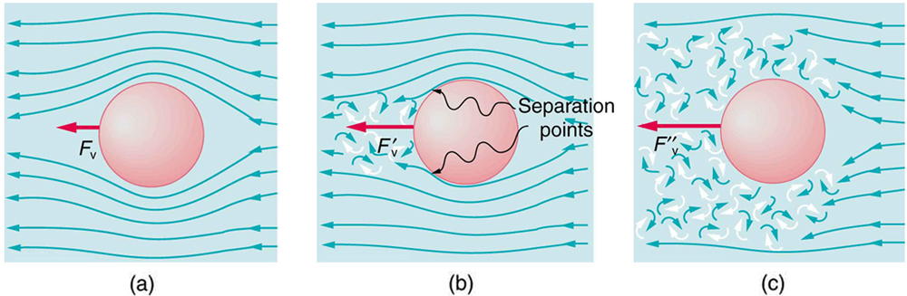
This formula assumes that the flow around the object is laminar (smooth) and that inertial effects are negligible compared to viscous effects – conditions that are characterized by low Reynolds numbers.
Derivation and Assumptions
Stokes’ Law was developed under specific assumptions that define the limits of its applicability:
Assumptions
- Spherical Particles: The law applies specifically to objects that are spherical. For non-spherical objects, deviations can occur and require additional correction factors.
- Laminar Flow: It is assumed that the movement of the particle results in a smooth, laminar flow in the surrounding fluid. This condition holds when the Reynolds number is sufficiently low, ensuring that turbulent effects can be neglected.
- Negligible Inertia: The derivation of the law presumes that inertial forces are much smaller than the viscous forces acting on the particle. This is the case when particles move slowly through the fluid.
Physical Reasoning
The derivation of Stokes’ Law involves using the Navier-Stokes equations under the assumption of steady, incompressible, and low Reynolds number flow conditions. By solving these equations around a sphere, one can arrive at an expression for the drag force that incorporates the radius, fluid viscosity, and the velocity of the sphere. In essence, the formula shows that the drag force increases linearly with the radius and velocity of the sphere, as well as with the viscosity of the fluid. The proportional constant, \(6\pi\), comes from the geometric and mathematical specifics of a sphere.
This linear relationship is particularly valuable because it provides a method to experimentally measure the viscosity of fluids by observing the terminal velocity of spheres falling through the medium, a method illustrated famously in Millikan's oil drop experiment.
Practical Applications of Stokes’ Formula
Stokes’ Law finds a multitude of applications across various fields, including:
Measuring Fluid Viscosity
One of the most straightforward applications of Stokes’ formula is in determining the viscosity of a liquid. By releasing a spherical particle into the fluid and measuring its terminal velocity (the constant velocity it reaches when the drag force equals the gravitational force), one can rearrange the formula to solve for the viscosity \( \eta \):
\( \eta = \dfrac{F}{6\pi r v} \)
In practice, once the drag force is balanced by gravitational and buoyant forces, the terminal velocity provides a clear means to back-calculate the viscosity. This technique has significant importance in both lab-scale measurements and industrial applications.
Sedimentation and Particle Settling
The law also plays a critical role in understanding sedimentation. In natural water bodies and engineered processes, particles settle under gravity. Stokes’ Law predicts the settling velocity of these particles, which aids in the design of sedimentation tanks, analysis of pollutant dispersion, and even in the study of blood cells in biophysics.
Biomedical Applications
In biomedical contexts, Stokes’ formula helps analyze the behavior of cells or micro-particles suspended in bodily fluids. The controlled motion of these particles under known force conditions contributes to advances in diagnostics and targeted drug delivery systems.
Environmental and Industrial Processes
Environmental scientists employ the formula to predict and model the behavior of pollutants in atmospheric and aquatic environments. Similarly, industries involved in chemical processing use Stokes’ Law to design systems where particulate matter is separated from fluids, ensuring efficient processing and minimal waste.
Comparative Overview: Stokes’ Law vs. Stokes’ Theorem
Although the term “Stokes formula” is most frequently denoting the drag force equation described above, it is important to differentiate it from Stokes’ Theorem—a fundamentally different concept in vector calculus. Stokes’ Theorem relates a surface integral over a surface to a line integral around its boundary, expressed as:
\( \oint_C \mathbf{F} \cdot d\mathbf{r} = \iint_S (\nabla \times \mathbf{F}) \cdot d\mathbf{S} \)
This theorem is a cornerstone of mathematical physics, particularly in the analysis of electromagnetic fields and fluid flows. While both concepts bear the name "Stokes," they apply to very different problems and domains. Stokes’ Law is used to understand forces on particles in fluids, whereas Stokes’ Theorem is used to convert between different forms of integrals in vector calculus.
It is crucial to recognize the contextual applications when one encounters the term "Stokes formula." In fields tied to fluid dynamics, the drag force formula is almost always the subject of discussion. In contrast, in mathematics and physics contexts discussing fields and circulation, Stokes’ Theorem is the likely reference.
Detailed Mathematical Explanation
For those interested in the mathematical rigor behind Stokes’ Law, here is a higher-level breakdown of the derivation process under ideal conditions:
| Parameter | Symbol | Physical Meaning |
|---|---|---|
| Drag Force | \( F \) | Force resisting the motion of the sphere |
| Viscosity | \( \eta \) | Dynamic viscosity of the fluid |
| Sphere Radius | \( r \) | Radius of the spherical particle |
| Velocity | \( v \) | Relative velocity of the particle |
The derivation stems from solving the Navier-Stokes equations under the conditions of steady, incompressible flow. By considering the symmetry of the sphere, boundary conditions (which include the no-slip condition at the sphere’s surface), and the decreasing effect of the velocity at large distances, the complete derivation leads to the equation:
\( F = 6 \pi \eta r v \)
The constant \(6\pi\) emerges from the integration of the viscous stress components over the sphere’s surface. Every parameter in this equation plays a role in overcoming the viscous drag imposed by the fluid's resistance to deformation.
Extensions and Limitations
While the formula provides significant predictive power, certain limitations and extensions should be kept in mind:
Extensions
In cases where the assumptions of spherical shape and laminar flow do not hold precisely, researchers may introduce modifications. For nonspherical objects or higher Reynolds numbers, empirical or semi-empirical corrections are used to adjust the formula. Additionally, when multiple particles interact or when boundary effects (such as walls) become significant, the simple form of Stokes’ Law might require further refinement.
Limitations
Stokes’ Law is strictly valid under the assumption of low Reynolds numbers, where the inertial forces are negligible relative to viscous forces. In turbulent conditions or when particles are large enough that inertial effects become significant, the drag-force relationship deviates markedly from the predictions of this law. Engineers and scientists must thus carefully consider the flow regime when applying Stokes’ Law in practical scenarios.
Furthermore, the law assumes an infinite and homogeneous fluid. In real applications, factors such as fluid boundaries and variations in fluid properties might require additional corrections to the ideal equation.
Visualization and Example
To illustrate the application of Stokes’ Law, consider the following example. Imagine a small spherical particle falling under gravity through a viscous liquid. As the particle accelerates, the increasing drag force eventually balances the net gravitational force (taking into account buoyancy). At this point, the particle reaches its terminal velocity, \( v_t \), and continues to fall at a constant speed.
Using Stokes’ Law, one can determine the drag force at terminal velocity, which then helps calculate the viscosity of the fluid if the other parameters (radius and velocity) are measured. Such an experimental setup is used widely in research laboratories to determine fluid properties.
Here is a simplified step-by-step outline:
- Measure the radius \( r \) of the spherical particle.
- Allow the particle to fall through the fluid until it reaches terminal velocity \( v_t \).
- Calculate the drag force \( F \) using the balance of forces (gravitational minus buoyant force equals drag force).
- Apply Stokes’ Law to solve for the dynamic viscosity \( \eta \).
This controlled experiment vividly demonstrates how theoretical predictions translate into practical measurements.
Beyond the Basics: Broader Impact of Stokes’ Formula
The influence of Stokes’ formula extends beyond simple fluid dynamics. Its impact is felt across multiple disciplines:
In Physics and Engineering
In physics, the ability to predict drag forces with great accuracy is vital for understanding particle motion, aerosol dynamics, and even astrophysical phenomena where small particles interact with gaseous media. Engineers incorporate these principles into the design of systems for particle separation and in the development of instruments that measure fluid properties.
In Environmental Science
Environmental researchers apply Stokes’ Law when modeling sediment transport in rivers, lakes, and estuaries. Predicting the settling velocity of particles allows for better management of natural resources and designing interventions to mitigate pollution.
In Medical Diagnostics
The principles underlying Stokes’ formula are used in designing medical devices that rely on the controlled movement of tiny particles, such as in blood flow diagnostics and drug delivery systems. Accurate control of particle motion at micro scales aids in developing targeted treatments and diagnostic tools.
The theoretical underpinning provided by Stokes’ Law remains a cornerstone of experimental design. Its proficiency in bridging theoretical physics with experimental observations underscores its enduring relevance in both academic research and practical applications.
Advanced Practical Considerations
While the clean mathematically derived form of Stokes’ Law provides a useful tool for understanding drag forces, various practical considerations must be taken into account:
- Temperature Effects: Since fluid viscosity is temperature-dependent, variations in the ambient temperature can affect the measured drag force. It is essential to maintain temperature control during experiments.
- Particle Interactions: In systems where multiple particles are present, interactions between particles may modify the effective drag experienced by each one.
- Boundary Effects: The proximity of walls or other boundaries in the experimental setup can modify the flow profile around a particle. Correction factors are often applied to account for these influences.
Engineers and researchers often simulate these conditions using computational fluid dynamics (CFD) models to predict deviations from the ideal case. Such simulations improve the applicability of Stokes’ Law in complex real-world scenarios.
Final Thoughts on Stokes Formula
Stokes’ formula, particularly in its form as Stokes’ Law, is a fundamental and widely used relation in fluid dynamics. This formula not only allows us to compute the drag force on spherical particles moving through a viscous medium but also serves as a building block in many applied sciences. By understanding the principles underlying this law, one appreciates the delicate balance of forces in fluid systems and the interplay between theoretical physics and experimental measurements.
It is this blend of theory and practice that makes Stokes’ Law such a rich subject of study and application. Whether you are a student encountering these principles for the first time or a seasoned professional employing them in a research or engineering context, the precision and utility offered by Stokes’ formula continue to inspire curiosity and technological innovation.
References
- Stokes's law | Definition, Formula, & Facts - Britannica
- Stoke's Law: Definition, Derivation, Formula & Solved Examples - GeeksforGeeks
- Stokes' law - Wikipedia
- Stokes Law Derivation - BYJU'S
- Stokes' Law: Statement, Formula, Assumptions & Limitations - Science Facts
-
Stokes’ formula - ScienceDirect
- What is Stokes Law? - Trucent
- Stokes' Theorem - LibreTexts
- Stokes Theorem - BYJU'S
- Stokes' Law Overview - Science Facts
Recommended Related Queries
Last updated March 2, 2025