The quest to accurately simulate fluid dynamics using the Navier-Stokes equations via Finite Element Analysis (FEA) is a cornerstone of modern engineering and physics. Traditional Adaptive Mesh Refinement (AMR) techniques have long been used to improve accuracy by concentrating computational effort where it's needed most. However, the integration of Machine Learning (ML) promises a paradigm shift, potentially offering significantly more efficient and accurate meshing strategies. Based on the conceptual framework presented in cutting-edge research, let's explore the mathematical architecture required to formally prove the enhanced error bounds achievable with ML-driven AMR specifically for the challenging Navier-Stokes equations.

Highlights: The Core Arguments

• Proving Superiority: The central goal is to mathematically demonstrate that ML-enhanced AMR yields tighter error bounds (e.g., \( E_{ML}(N) < E_{Trad}(N) \)) or achieves faster convergence rates (\( \alpha_{ML} > \alpha_{Trad} \)) compared to traditional methods for Navier-Stokes FEA, given the same computational cost \(N\).
• Multi-Disciplinary Framework: Constructing such proofs requires integrating concepts from numerical analysis (FEA theory, a posteriori error estimation, stability analysis), approximation theory, and machine learning theory (statistical learning, reinforcement learning convergence).
• Navier-Stokes Complexity: The inherent non-linearity, coupled velocity-pressure fields, and potential for complex phenomena like turbulence and singularities in Navier-Stokes flows add significant layers of difficulty to the theoretical analysis.

---

Setting the Stage: Navier-Stokes and FEA Fundamentals

Understanding the Equations and the Measurement of Success

Before delving into the proofs, we must define the problem context and the metrics used to evaluate success.

The Navier-Stokes Equations

For an incompressible, viscous fluid in a domain \( \Omega \subset \mathbb{R}^d \) (typically \(d=2\) or \(3\)), the steady-state Navier-Stokes equations are given by:

\[ \begin{aligned} -\nu \Delta \mathbf{u} + (\mathbf{u} \cdot \nabla) \mathbf{u} + \nabla p &= \mathbf{f} \quad &\text{in } \Omega, \ \nabla \cdot \mathbf{u} &= 0 \quad &\text{in } \Omega, \ \mathbf{u} &= \mathbf{g} \quad &\text{on } \partial \Omega. \end{aligned} \] Here, \( \mathbf{u} \) represents the fluid velocity field, \( p \) is the pressure, \( \nu > 0 \) is the kinematic viscosity, \( \mathbf{f} \) is an external body force, and \( \mathbf{g} \) represents prescribed boundary conditions. The non-linear term \( (\mathbf{u} \cdot \nabla) \mathbf{u} \) makes these equations particularly challenging to solve analytically and numerically.

Finite Element Analysis (FEA) Context

FEA tackles these equations by discretizing the domain \( \Omega \) into a mesh of smaller elements (like triangles or tetrahedra) and approximating the continuous solution fields \( (\mathbf{u}, p) \) with piecewise polynomial functions \( (\mathbf{u}_h, p_h) \) defined over this mesh. The accuracy of the approximation \( (\mathbf{u}_h, p_h) \) heavily depends on the quality and resolution of the mesh.

Quantifying Error and Cost

To compare different meshing strategies, we need precise metrics:

• Error (E): The discrepancy between the true solution \( (\mathbf{u}, p) \) and the FEA approximation \( (\mathbf{u}_h, p_h) \). This is typically measured using mathematical norms. Common choices for Navier-Stokes include:
  • Energy Norm: Captures errors in both the solution and its gradients (related to viscous stresses). A typical form might be: \[ \| (\mathbf{u} - \mathbf{u}_h, p - p_h) \|_{\text{Energy}} \approx \left( \nu \|\nabla (\mathbf{u} - \mathbf{u}_h)\|_{L^2(\Omega)}^2 + \| \dots \| \right)^{1/2} \] (The exact form depends on the specific FE formulation).
  • L² Norm: Measures the average magnitude of the error: \[ \| \mathbf{u} - \mathbf{u}_h \|_{L^2(\Omega)} = \left( \int_{\Omega} |\mathbf{u}(x) - \mathbf{u}_h(x)|^2 dx \right)^{1/2} \] Similar norms apply to the pressure error \( \| p - p_h \|_{L^2(\Omega)} \).
• Computational Cost (C): Usually measured by the number of elements \( N \) in the mesh, or equivalently, the total number of degrees of freedom (DoFs) in the system. Cost impacts simulation time and memory requirements.

The overarching goal of any adaptive meshing strategy is to minimize the error \( E \) for a given computational cost budget \( C \), or achieve a target error tolerance \( \epsilon \) with the minimum possible cost.

---

The Benchmark: Traditional Adaptive Mesh Refinement (AMR)

Established Techniques and Their Theoretical Limits

Traditional AMR methods iteratively refine the mesh based on feedback from the computed solution. The core idea is to add more elements (increase resolution) in regions where the estimated error is high.

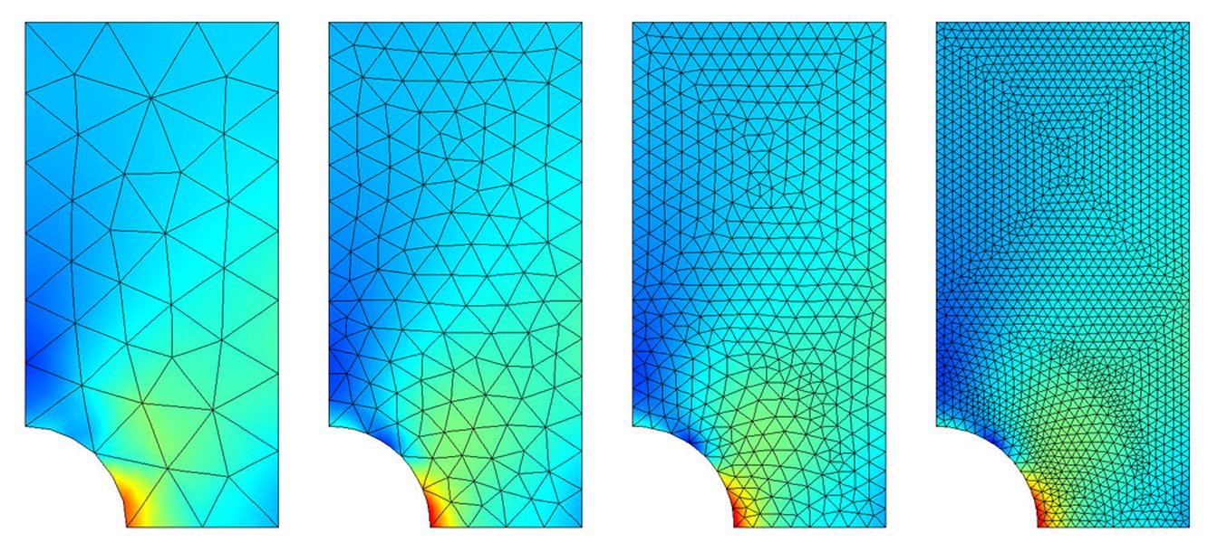
Adaptive mesh refinement focusing elements in areas of high solution variation.

A Posteriori Error Estimation

These methods rely on a posteriori error estimators, denoted by \( \eta \). These are computable quantities based on the approximate solution \( (\mathbf{u}_h, p_h) \) that provide an estimate of the true error \( E \). A common form is a global estimator composed of local (element-wise) indicators \( \eta_K \):

\[ \eta = \left( \sum_{K \in \mathcal{T}_h} \eta_K^2 \right)^{1/2} \] The local indicators \( \eta_K \) typically involve residuals of the PDE within element \( K \) and jumps in the solution derivative across element edges. Theoretical guarantees link the estimator to the true error:

• Reliability: \( E \leq C_{rel} \eta \) (The estimator provides an upper bound on the true error).
• Efficiency: \( \eta \leq C_{eff} (E + \text{osc}) \) (The estimator is bounded by the true error, up to data oscillations).

Refinement Strategy and Convergence

A typical AMR algorithm follows a loop: SOLVE \(\rightarrow\) ESTIMATE \(\rightarrow\) MARK \(\rightarrow\) REFINE.

1. Compute \( (\mathbf{u}_h, p_h) \) on the current mesh \( \mathcal{T}_h \).
2. Calculate the error indicators \( \eta_K \) for all elements \( K \).
3. Mark elements with the largest \( \eta_K \) for refinement (e.g., using a fixed fraction or Dörfler marking).
4. Refine the marked elements (e.g., by subdividing them).

Under certain assumptions (e.g., mesh regularity, estimator properties), traditional AMR can achieve theoretically optimal convergence rates for certain problem classes. For a solution with sufficient regularity, the error often behaves like:

\[ E(N) \leq K_{Trad} N^{-\alpha_{Trad}} \] where \( N \) is the number of DoFs, \( K_{Trad} \) is a constant, and \( \alpha_{Trad} > 0 \) is the convergence rate (e.g., \( \alpha_{Trad} \approx p/d \) for polynomial degree \( p \) and dimension \( d \)). However, the heuristics used for marking might not always lead to the truly optimal mesh distribution, especially for complex, non-linear problems like Navier-Stokes.

Comparison showing how adaptive refinement (right) uses elements more efficiently than uniform refinement (left).

---

Introducing Intelligence: ML-Enhanced AMR Strategies

Leveraging Data and Learning for Smarter Meshing

ML-enhanced AMR aims to replace or augment the heuristic "MARK" step of traditional AMR with a learned strategy. The idea is that ML models can potentially learn more complex relationships between the solution state and the optimal mesh configuration, leading to better performance.

Modeling the ML Approach

Two common approaches emerge:

1. Predictive Models: Train an ML model (e.g., a Convolutional Neural Network - CNN) to directly predict an optimal mesh density function \( f_{ML}: \Omega \rightarrow \mathbb{R}^+ \), which specifies the desired local element size \( h(x) \) at each point \( x \) in the domain. The mesh generation algorithm then attempts to create a mesh respecting this density. The model is typically trained on data from previous simulations or known optimal meshes.
2. Reinforcement Learning (RL): Frame mesh adaptation as a sequential decision-making problem. An RL agent learns a policy \( \pi_{ML} \) that takes the current state (mesh, solution \( (\mathbf{u}_h, p_h) \), geometry) and outputs refinement/coarsening actions for different parts of the mesh. The agent is trained by maximizing a reward function that balances error reduction and computational cost, e.g., \( R_t = -(\lambda_E E_t + \lambda_C C_t) \), where \( \lambda_E, \lambda_C \) are weights.

The Potential Advantage

ML models, especially deep neural networks, can potentially capture highly non-linear and non-local dependencies in the data. For Navier-Stokes, this could mean:

• Better prediction of where complex flow features (vortices, boundary layers, shocks) will form or propagate.
• Learning implicit correlations between different parts of the flow field that traditional local estimators might miss.
• Optimizing the mesh globally to satisfy theoretical conditions like the equidistribution principle (where local error indicators \( \eta_K \) are roughly equal across all elements) more effectively than heuristic marking.

Visualizing the ML-AMR Framework

This mindmap illustrates the key components involved in establishing the mathematical proof for ML-enhanced AMR in the context of Navier-Stokes FEA:

---

Constructing the Mathematical Proof

Combining Numerical Analysis and Learning Theory

A rigorous proof demonstrating \( E_{ML}(N) < E_{Trad}(N) \) or \( \alpha_{ML} > \alpha_{Trad} \) for Navier-Stokes is not a single formula but a structured argument built upon several theoretical pillars.

1. A Posteriori Error Bounds for Navier-Stokes FEA

The foundation relies on established a posteriori error estimation theory for the specific FEA discretization used for Navier-Stokes (e.g., stabilized methods like SUPG/PSPG, or mixed methods satisfying the inf-sup condition). These provide the reliable and efficient estimator \( \eta \) linked to the true error \( E \).

\[ E \approx \eta = \left( \sum_{K \in \mathcal{T}_h} \eta_K^2 \right)^{1/2} \] The local indicators \( \eta_K \) typically depend on element-wise residuals of the momentum and continuity equations, plus jump terms across element interfaces.

2. Approximation Theory and Optimal Meshes

Standard FEA interpolation theory states that the error on an element \( K \) is related to the mesh size \( h_K \) and derivatives of the true solution \( \mathbf{u} \):

\[ \| \mathbf{u} - I_h \mathbf{u} \|_{L^2(K)} \leq C h_K^{p+1} \| D^{p+1} \mathbf{u} \|_{L^2(K)} \] (assuming polynomial degree \( p \)). Optimal meshes aim to distribute the elements such that the local errors are balanced (equidistribution principle), often meaning \( h_K \) should be smaller where derivatives \( \| D^{p+1} \mathbf{u} \| \) are large. The proof must argue that the ML strategy (either predicting \( h(x) \) or the RL policy actions) generates meshes that are closer to this theoretical optimum compared to traditional heuristics. This involves showing that the ML approach better approximates the ideal mesh size function \( h^*(x) \), potentially leveraging monitor functions or metric tensors \( M(x) \) derived from solution features.

Let \( h_{ML}(x) \) be the mesh size produced by the ML strategy and \( h_{Trad}(x) \) by the traditional one. A key step is to show:

\[ \| h_{ML} - h^* \|_{L^p(\Omega)} < \| h_{Trad} - h^* \|_{L^p(\Omega)} \] for some suitable norm, implying \( h_{ML} \) is a better approximation of the ideal mesh size \( h^* \). This improved approximation, plugged back into the error bounds, leads to a smaller overall error \( E_{ML} \).

3. Stability Considerations (Inf-Sup Condition)

For Navier-Stokes FEA using mixed formulations (approximating \( \mathbf{u} \) and \( p \) in different spaces \( V_h \) and \( Q_h \)), stability requires satisfying the Ladyzhenskaya-Babuška-Brezzi (LBB) or inf-sup condition:

\[ \inf_{q_h \in Q_h} \sup_{\mathbf{v}_h \in V_h} \frac{\int_{\Omega} q_h (\nabla \cdot \mathbf{v}_h) dx}{\| q_h \|_{Q} \|\mathbf{v}_h\|_{V}} \geq \beta > 0 \] where \( \beta \) must be independent of the mesh size \( h \). The proof must ensure that the mesh sequences generated by the ML-AMR strategy do not violate this condition, which could lead to spurious pressure oscillations. This might involve constraints on element shapes (e.g., aspect ratios) or specific refinement rules compatible with stability preservation.

4. Learning Theory Guarantees

Since the ML strategy is learned from data, the proof needs to incorporate arguments from learning theory:

• Generalization Bounds (for predictive models): Using tools like VC-dimension or Rademacher complexity from statistical learning theory, one needs to show that the ML model's performance (e.g., accuracy in predicting \( h^*(x) \)) observed on the training data generalizes well to new, unseen Navier-Stokes problems. This provides confidence that the error bounds hold beyond the training set. \[ \mathbb{E}_{\text{new data}} [ \text{Error}(ML) ] \leq \text{Error}_{\text{train}}(ML) + \epsilon_{gen}(\text{complexity}, N_{\text{train}}) \]
• Policy Convergence (for RL models): If using RL, the proof must leverage theorems from RL theory (e.g., for policy gradient or Q-learning) demonstrating that the learned policy \( \pi_{ML} \) converges towards an optimal policy \( \pi^* \) that truly minimizes the long-term error-cost objective function.

5. Synthesizing the Argument for Improved Bounds/Rates

The final step combines these elements. By showing that the ML strategy (proven to generalize or converge) generates stable meshes that better approximate the optimal mesh distribution (closer to \( h^* \)), leveraging approximation theory bounds linked to a posteriori estimates, one can conclude that for a given \( N \), \( E_{ML} \leq C_{ML} N^{-\alpha_{ML}} \) where \( C_{ML} \leq C_{Trad} \) and \( \alpha_{ML} \geq \alpha_{Trad} \), with at least one inequality being strict under conditions where ML significantly improves upon heuristics (e.g., complex flows with interacting features).

---

Comparing Approaches: Traditional vs. ML-Enhanced AMR

A Hypothetical Performance Snapshot

While rigorous proofs are challenging, we can visualize the *expected* relative strengths and weaknesses based on the theoretical potential. The following chart provides a hypothetical comparison across key performance dimensions for Navier-Stokes simulations.

This chart suggests that while ML-based methods hold the potential for superior convergence and efficiency, especially with RL's adaptive nature, they currently face challenges in implementation complexity and established theoretical guarantees compared to traditional AMR.

Tabular Comparison

Here's a summary table highlighting the key distinctions:

Feature	Traditional AMR	ML-Enhanced AMR
Refinement Driver	A posteriori error estimators (e.g., residuals, jumps)	Learned function (predicted density/error) or RL policy
Optimality Basis	Heuristics targeting error reduction (e.g., Dörfler marking)	Data-driven optimization of mesh properties, potentially closer to theoretical optimum (e.g., equidistribution)
Adaptability	Generally robust but may use conservative heuristics	Potentially highly adaptive to complex/non-linear features; performance depends on training data/process
Handling Complex Features	Reliant on estimator capturing the feature's impact on error	Can learn subtle correlations and predict feature evolution/location
Theoretical Maturity	Well-established convergence proofs for many cases	Active research area; proofs require integrating learning theory and are often method/problem specific
Implementation Effort	Standard libraries available; relatively straightforward	Requires ML expertise, data pipelines, training infrastructure; more complex integration

---

Computational Fluid Dynamics in Action

Visualizing the Application Domain

Understanding the complexity of fluid flows simulated using Navier-Stokes equations helps appreciate the need for advanced meshing techniques like ML-enhanced AMR. Computational Fluid Dynamics (CFD) is the field dedicated to these simulations, impacting diverse areas from aerospace engineering to weather forecasting. The video below provides a general overview of CFD simulation.

This video illustrates the typical workflow and visual outputs of CFD simulations, which often rely heavily on the underlying mesh quality generated by methods like FEA. Achieving accurate results for complex geometries and flow conditions, such as those shown, motivates the development of more intelligent meshing strategies.

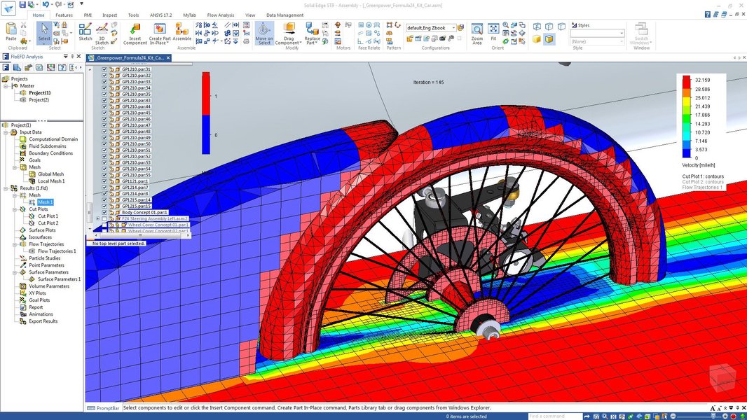
Example of CFD simulation results visualized in engineering software.

---

Challenges and the Road Ahead

Navigating the Complexities of Proof and Practice

While the framework exists, constructing a universally applicable, mathematically airtight proof that ML-AMR *always* outperforms traditional AMR for *any* Navier-Stokes problem is extremely challenging, perhaps impossible. Key hurdles include:

• Navier-Stokes Complexity: The non-linearity, potential for turbulence (requiring very fine scales or modeling), and sensitivity to boundary conditions make rigorous analysis difficult even for traditional methods.
• ML Model Dependency: The performance and theoretical guarantees depend heavily on the specific ML architecture, training data, and hyperparameters used. A proof might only hold for a particular class of models or training regimes.
• The "No Free Lunch" Theorems: These theorems in optimization and machine learning suggest that no single algorithm is optimal across all possible problems. An ML strategy excelling at one type of flow might perform poorly on another if not trained broadly.
• Combining Theories: Seamlessly integrating the guarantees from numerical analysis (related to PDE properties) with those from learning theory (related to data and algorithms) is a complex theoretical task.
• Stability Guarantees: Ensuring the ML-generated meshes consistently satisfy stability conditions like the inf-sup condition requires careful design or analysis.

Current research focuses on proving performance improvements for specific classes of problems, particular ML approaches, or under certain assumptions about the solution's regularity or the quality of the training data.

---

Frequently Asked Questions (FAQ)

Clarifying Key Aspects

---

References

Further Reading and Sources

The synthesis presented here draws upon concepts discussed in the provided answers and general principles from numerical analysis and machine learning. Key referenced ideas and related background can be explored further via:

• Can Machine Learning Truly Revolutionize Finite Element Meshing? Unpacking the Mathematical Proof - Ithy (Conceptual Framework Source)
• Analysis Of The Finite Element Method - Norms Lesson 1 - Ansys Innovation Space (FEA Norms & Convergence)
• Practical Finite Element Analysis (FEA) — A Guide - fiveflute (FEA Fundamentals)
• Errors in FEA and Understanding Singularities - SimScale (FEA Errors & Meshing)
• Common Errors in Finite Element Analysis and How To Avoid Them - Structures Centre (Mesh Quality)
• Navier–Stokes equations - Wikipedia (Equation Fundamentals)
• Error-bounds for finite element method - European Digital Mathematics Library (FEA Error Bounds)
• Mathematical Analysis of the Navier-Stokes Equations - Springer (Navier-Stokes Analysis)

---

Recommended

Explore Related Concepts