
Unveiling the Financial Ripple Effect: How Different Depreciation Methods Shape Business Performance
A deep dive into Straight-Line, Declining Balance, and other methods, revealing their distinct impacts on income, taxes, and asset valuation.
Depreciation, a fundamental accounting concept, signifies the systematic allocation of a tangible asset's cost over its expected useful life. It's not just an accounting entry; it's a critical factor influencing a company's reported profitability, tax obligations, and overall financial picture. The method chosen to calculate depreciation can significantly alter these financial outcomes. This study undertakes a comparative analysis of various depreciation methods to illuminate their distinct impacts on financial performance.
Key Insights at a Glance
- Depreciation Method Matters: The choice between methods like Straight-Line, Double-Declining Balance, Sum-of-Years-Digits, and Units of Production directly impacts reported net income, asset book values on the balance sheet, and tax liabilities.
- Timing is Everything: Accelerated methods (Double-Declining Balance, Sum-of-Years-Digits) front-load depreciation expense, reducing taxable income and taxes in early years but lowering reported profits, while the Straight-Line method provides consistency.
- Strategic Choice: Selecting a depreciation method should align with a company's asset usage patterns, financial reporting goals, tax strategy, and industry norms.
Why Study Depreciation Methods? The Need Explored
Understanding the Financial Undercurrents
The need for this comparative study stems from the significant and varied effects depreciation methods have on a company's financial health. Depreciation expense flows through the income statement, reducing net income. It also impacts the balance sheet by decreasing the carrying value (book value) of assets over time. While depreciation is a non-cash expense, its influence on taxable income directly affects cash flows through tax payments. Different methods result in different patterns of expense recognition, influencing:
- Profitability Metrics: Net income, operating income, and related ratios (like Return on Assets) change depending on the depreciation expense recorded each period.
- Tax Liabilities: Accelerated methods can defer tax payments by recognizing higher expenses in earlier years, impacting cash flow planning. Awareness of changing regulations, like the reduction in bonus depreciation rates for 2024-2025, is crucial.
- Asset Valuation: The book value of assets declines differently under various methods, affecting balance sheet ratios (e.g., debt-to-equity) and potentially influencing investor perception and business valuation.
- Investment Decisions: The timing of depreciation expense can influence decisions about acquiring new assets or replacing old ones.
Given these wide-ranging impacts, a thorough understanding and comparison of depreciation methods are essential for accurate financial reporting, effective tax planning, strategic asset management, and informed decision-making by stakeholders.
Depreciation analysis is a key component of comprehensive financial statement analysis.
Objectives of the Study
Defining Our Analytical Goals
The primary objectives guiding this comparative study are:
- To explain the concept of depreciation and its fundamental importance in financial accounting.
- To describe and detail the calculation mechanics of common depreciation methods: Straight-Line (SL), Double-Declining Balance (DDB), Sum-of-the-Years' Digits (SYD), and Units of Production (UOP).
- To conduct a comparative analysis of how applying these different methods impacts a company's key financial statements (Income Statement, Balance Sheet, Cash Flow Statement).
- To evaluate the effect of each depreciation method on crucial financial performance indicators and ratios (e.g., net income, asset book value, return on assets).
- To examine the tax implications associated with different depreciation strategies, particularly the benefits and drawbacks of accelerated depreciation.
- To provide insights and suggestions for businesses on selecting the most appropriate depreciation method based on their specific circumstances and strategic objectives.
Scope and Boundaries
Defining the Analytical Arena
The scope of this study encompasses:
- A focus on the four most widely recognized depreciation methods allowed under Generally Accepted Accounting Principles (GAAP): Straight-Line, Double-Declining Balance, Sum-of-the-Years' Digits, and Units of Production.
- Analysis limited to tangible fixed assets (e.g., machinery, equipment, buildings, vehicles). Intangible asset amortization is excluded.
- Examination of the impact on financial performance using a hypothetical company profile within the manufacturing sector as a case study.
- Assessment of effects on the primary financial statements and related financial ratios over the asset's useful life.
- Consideration of U.S. GAAP context and general tax implications, acknowledging recent changes like the bonus depreciation phase-down.
Acknowledging the Limitations
Understanding the Constraints
This study is subject to certain limitations:
- Data Source: The analysis relies on a hypothetical company profile and generalized examples derived from secondary sources, not real-world, company-specific proprietary data.
- Generalizability: Findings based on a single hypothetical manufacturing company may not be directly applicable to all companies or industries, especially those with vastly different asset structures (e.g., service industries, energy sector).
- Simplifying Assumptions: The analysis assumes constant variables like useful life and salvage value, which can change in reality due to unforeseen circumstances or revised estimates. Asset impairments are not considered.
- External Factors: The study does not incorporate the impact of broader economic conditions, market fluctuations, or specific technological obsolescence rates that can affect asset values and depreciation in practice.
- Regulatory Dynamics: While acknowledging recent changes, the study cannot predict future alterations in accounting standards or tax laws related to depreciation.
Research Methodology: Our Approach
Structuring the Investigation
Research Design
This study utilizes a descriptive and comparative analytical research design. It aims to describe the characteristics and mechanics of different depreciation methods and comparatively analyze their quantitative impact on financial statements and performance metrics using a case study approach.
Sampling Size and Procedure
The study focuses on a single hypothetical case – a manufacturing company ("ManuCorp") and a specific asset (machinery). This purposive selection allows for an in-depth comparison of depreciation methods applied to the same asset base, rather than a statistical sampling of multiple companies. The asset details are: Cost = $100,000, Salvage Value = $10,000, Useful Life = 5 years, Total Expected Production = 20,000 units.
Data Collection Method
Data collection relies exclusively on secondary sources. This includes information synthesized from the provided answers (which reference accounting principles, financial guides, and articles) and established accounting formulas for depreciation calculation. No primary data (interviews, surveys) was collected.
Data Analysis Tools
The primary tools for data analysis are:
- Spreadsheet Software (e.g., Excel): Used for calculating depreciation schedules year-by-year for each method based on standard formulas.
- Comparative Analysis: Comparing the annual depreciation expense, accumulated depreciation, and resulting book value across the different methods.
- Financial Statement Impact Assessment: Interpreting how the differing depreciation expenses would affect net income, taxes (qualitatively), and asset values on hypothetical financial statements.
- Ratio Analysis (Conceptual): Discussing how key ratios like Net Profit Margin and Return on Assets would likely be affected by the choice of method.
Industry and Company Profile
Setting the Stage: ManuCorp
To illustrate the comparative analysis, we consider ManuCorp, a hypothetical mid-sized company operating in the machinery and equipment manufacturing industry. This sector is typically capital-intensive, with significant investments in tangible assets like production machinery, plants, and vehicles, making depreciation a highly relevant accounting issue.
On January 1, 2025, ManuCorp purchases a new piece of specialized manufacturing machinery with the following characteristics:
- Asset Cost: $100,000
- Estimated Useful Life: 5 years
- Estimated Salvage Value: $10,000
- Estimated Total Production Capacity: 20,000 units
- Estimated Annual Production (for UOP method): Year 1: 4,000 units, Year 2: 5,000 units, Year 3: 4,500 units, Year 4: 3,500 units, Year 5: 3,000 units
This profile provides the basis for calculating and comparing depreciation under different methods.
Companies must choose appropriate depreciation methods for diverse assets like machinery, vehicles, and buildings.
Data Analysis and Interpretation: Crunching the Numbers
Comparing Depreciation Schedules and Financial Impacts
Using ManuCorp's machinery purchase details, we calculate the annual depreciation expense for the 5-year useful life under four common methods: Straight-Line (SL), Double-Declining Balance (DDB), Sum-of-the-Years' Digits (SYD), and Units of Production (UOP).
Depreciation Calculations
1. Straight-Line (SL):
\[ \text{Annual Depreciation} = \frac{\text{Cost} - \text{Salvage Value}}{\text{Useful Life}} = \frac{\$100,000 - \$10,000}{5} = \$18,000 \]The depreciation expense is a constant $18,000 each year.
2. Double-Declining Balance (DDB):
\[ \text{SL Rate} = \frac{1}{\text{Useful Life}} = \frac{1}{5} = 20\% \] \[ \text{DDB Rate} = 2 \times \text{SL Rate} = 40\% \] \[ \text{Depreciation (Year)} = \text{Beginning Book Value} \times \text{DDB Rate} \]Note: Depreciation stops when Book Value reaches Salvage Value. The method may switch to SL in later years if DDB calculates depreciation below the SL amount needed to reach salvage value. The calculation below does not depreciate below the salvage value.
- Year 1: $100,000 * 40% = $40,000 (Book Value: $60,000)
- Year 2: $60,000 * 40% = $24,000 (Book Value: $36,000)
- Year 3: $36,000 * 40% = $14,400 (Book Value: $21,600)
- Year 4: $21,600 * 40% = $8,640 (Book Value: $12,960)
- Year 5: $12,960 - $10,000 = $2,960* (Depreciation limited to reach salvage value) (Book Value: $10,000)
- *Total DDB Depreciation: $40,000 + $24,000 + $14,400 + $8,640 + $2,960 = $90,000*
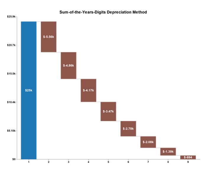
3. Sum-of-the-Years' Digits (SYD):
\[ \text{SYD Denominator} = 5 + 4 + 3 + 2 + 1 = 15 \] \[ \text{Depreciable Base} = \text{Cost} - \text{Salvage Value} = \$90,000 \] \[ \text{Depreciation (Year)} = \left( \frac{\text{Remaining Useful Life}}{\text{SYD Denominator}} \right) \times \text{Depreciable Base} \]- Year 1: (5/15) * $90,000 = $30,000
- Year 2: (4/15) * $90,000 = $24,000
- Year 3: (3/15) * $90,000 = $18,000
- Year 4: (2/15) * $90,000 = $12,000
- Year 5: (1/15) * $90,000 = $6,000
- *Total SYD Depreciation: $90,000*
4. Units of Production (UOP):
\[ \text{Depreciation Rate per Unit} = \frac{\text{Cost} - \text{Salvage Value}}{\text{Total Estimated Production}} = \frac{\$90,000}{20,000 \text{ units}} = \$4.50/\text{unit} \] \[ \text{Depreciation (Year)} = \text{Actual Units Produced} \times \text{Rate per Unit} \]- Year 1: 4,000 units * $4.50 = $18,000
- Year 2: 5,000 units * $4.50 = $22,500
- Year 3: 4,500 units * $4.50 = $20,250
- Year 4: 3,500 units * $4.50 = $15,750
- Year 5: 3,000 units * $4.50 = $13,500
- *Total UOP Depreciation: $90,000*
Comparative Table of Annual Depreciation Expense
This table summarizes the annual depreciation expense calculated under each method for ManuCorp's machinery. This comparison clearly illustrates the different patterns of expense recognition.
| Year | Straight-Line (SL) | Double-Declining Balance (DDB) | Sum-of-Years'-Digits (SYD) | Units of Production (UOP) |
|---|---|---|---|---|
| 1 | $18,000 | $40,000 | $30,000 | $18,000 |
| 2 | $18,000 | $24,000 | $24,000 | $22,500 |
| 3 | $18,000 | $14,400 | $18,000 | $20,250 |
| 4 | $18,000 | $8,640 | $12,000 | $15,750 |
| 5 | $18,000 | $2,960 | $6,000 | $13,500 |
| Total | $90,000 | $90,000 | $90,000 | $90,000 |
Interpretation of Financial Impacts
- Income Statement: Accelerated methods (DDB, SYD) report significantly higher depreciation expense in the early years (Year 1 DDB: $40k vs SL: $18k). This leads to lower reported net income and operating income initially, but higher income in later years compared to SL. UOP links expense directly to usage, causing income to fluctuate with production levels. SL provides the most stable impact on income over time.
- Balance Sheet: The asset's book value (Cost - Accumulated Depreciation) decreases fastest under DDB, followed by SYD, then SL and potentially UOP (depending on usage). A lower book value affects asset-based ratios. For example, at the end of Year 1, Book Value is $60k (DDB), $70k (SYD), $82k (SL & UOP).
- Cash Flow Statement: Depreciation is added back to net income in the operating activities section (indirect method) as it's a non-cash charge. However, the choice of method impacts cash flow indirectly through taxes. Higher depreciation expense (DDB, SYD in early years) means lower taxable income, resulting in lower income tax payments and thus higher operating cash flow in those initial years (tax shield effect). The total tax paid over the asset's life is theoretically the same, but the timing differs.
- Financial Ratios: Methods impact ratios differently. Early years under DDB/SYD show lower Profit Margins and Return on Assets (ROA) due to lower net income, but potentially higher Asset Turnover (Sales / Average Assets) due to lower average asset values. SL provides more stable ratios year-over-year.
Visualizing Depreciation Method Characteristics
Radar Chart Comparison
This chart provides a visual comparison of the four depreciation methods across several key characteristics. Higher scores indicate a stronger presence of that characteristic (e.g., higher first-year expense, greater income stability). This helps illustrate the trade-offs involved in selecting a method. Note that these scores represent relative comparisons based on the typical behavior of each method.
Mapping the Depreciation Landscape
Mindmap Overview
This mindmap provides a hierarchical overview of the depreciation methods discussed, their core principles, and key financial impacts. It serves as a quick reference guide to the concepts covered in this study.
Depreciation Methods"] id1["Straight-Line (SL)"] id1a["Principle: Equal expense annually"] id1b["Formula: (Cost - Salvage) / Life"] id1c["Impact: Stable Income,
Simple Calculation"] id2["Accelerated Methods"] id2a["Double-Declining Balance (DDB)"] id2a1["Principle: Highest expense early,
declines exponentially"] id2a2["Formula: Book Value * (2 / Life)"] id2a3["Impact: Early Tax Savings,
Lower Early Income"] id2b["Sum-of-Years-Digits (SYD)"] id2b1["Principle: High expense early,
declines linearly"] id2b2["Formula: Depreciable Base *
(Remaining Life / SYD)"] id2b3["Impact: Moderate Tax Savings,
Lower Early Income"] id3["Units of Production (UOP)"] id3a["Principle: Expense based on usage"] id3b["Formula: (Cost - Salvage) / Total Units *
Units Produced"] id3c["Impact: Matches expense to revenue,
Variable Income Impact"] id4["Financial Statement Impacts"] id4a["Income Statement:
Affects Net Income"] id4b["Balance Sheet:
Affects Book Value"] id4c["Cash Flow:
Indirect impact via Taxes"] id5["Key Considerations"] id5a["Tax Planning"] id5b["Financial Reporting Goals"] id5c["Asset Usage Pattern"] id5d["Industry Norms"]
Understanding Depreciation Methods Visually
Comparing Calculation Approaches
This video provides a helpful overview of different depreciation methods, including Straight-Line and Double-Declining Balance, explaining their core concepts and calculations. Watching this can reinforce the understanding of how these methods differ in allocating an asset's cost over time.
Video explaining various depreciation methods (Source: Corporate Finance Institute via YouTube).
Key Findings of the Study
Summarizing the Comparative Analysis
Based on the comparative analysis of the Straight-Line, Double-Declining Balance, Sum-of-Years-Digits, and Units of Production methods using the ManuCorp example, the following key findings emerge:
- Expense Recognition Pattern Varies Significantly: While the total depreciation expense over the asset's life ($90,000) is the same for SL, DDB, and SYD (and UOP if total estimated production is met), the timing of recognition differs dramatically. Accelerated methods (DDB, SYD) charge more expense early on, while SL charges a uniform amount. UOP fluctuates with activity.
- Impact on Reported Income: Accelerated methods result in lower reported net income in the early years and higher income in later years compared to the SL method. UOP's impact varies. This affects profitability analysis and trends.
- Tax Implications: The primary advantage of accelerated methods is tax deferral. By recognizing higher expenses earlier, companies can reduce their taxable income and thus pay less income tax in the initial years of an asset's life, improving near-term cash flow.
- Balance Sheet Values: Accelerated methods lead to a faster reduction in the asset's book value on the balance sheet. This impacts ratios involving total assets or fixed assets.
- Method Suitability:
- SL: Best for assets used evenly over time; simple, predictable. Preferred for financial reporting consistency.
- DDB/SYD: Suitable for assets that are more productive or efficient in early years, or prone to obsolescence. Offers tax advantages.
- UOP: Ideal for assets where usage varies significantly year-to-year (e.g., manufacturing equipment, vehicles based on mileage) as it best matches expense with revenue generation (matching principle).
- Choice is Strategic: The selection of a depreciation method is not merely an accounting compliance task but a strategic decision influencing financial reporting, tax management, and potentially investor perception.
Suggestions for Businesses
Making Informed Depreciation Choices
Based on the findings, businesses should consider the following when selecting and applying depreciation methods:
- Align Method with Asset Usage: Choose a method that genuinely reflects the pattern of the asset's economic benefit consumption. Use UOP if usage fluctuates heavily; consider SL for steady usage; evaluate accelerated methods if early productivity is higher or obsolescence is a risk.
- Consider Financial Reporting Objectives: If stable earnings are preferred for reporting purposes, SL might be suitable. If maximizing early-year tax deductions is a priority, accelerated methods are advantageous (often used for tax purposes even if SL is used for book purposes, creating deferred tax liabilities).
- Evaluate Tax Implications Carefully: Understand the cash flow benefits of tax deferral from accelerated methods, especially in the context of current tax laws and rates (including bonus depreciation rules).
- Maintain Consistency: Apply the chosen depreciation method consistently to similar classes of assets to ensure comparability over time, as required by GAAP. Changes in method require justification and disclosure.
- Enhance Disclosure: Clearly disclose the depreciation methods used for major asset classes in the financial statement footnotes, along with estimated useful lives and salvage values, to provide transparency to users.
- Regular Review: Periodically review the appropriateness of useful lives, salvage values, and even the depreciation method itself, especially if asset usage patterns or technology changes significantly.
Conclusion: The Significance of Depreciation Choices
Final Thoughts on Financial Performance Impact
Depreciation is far more than a routine accounting calculation; it is a critical element with a profound impact on a company's reported financial performance and position. This comparative study underscores that the choice of depreciation method—be it Straight-Line, Double-Declining Balance, Sum-of-the-Years' Digits, or Units of Production—materially affects the timing of expense recognition. This, in turn, influences reported net income, the carrying value of assets on the balance sheet, tax liabilities, and key financial ratios.
While all methods (except potentially UOP under fluctuating use) allocate the same total depreciable cost over an asset's life, the pattern of allocation varies significantly. Accelerated methods offer valuable tax deferral benefits, boosting early-year cash flows, but result in lower initial reported profits. The Straight-Line method provides simplicity and income statement stability, while the Units of Production method excels at matching costs with asset usage. Ultimately, the selection of a depreciation method requires careful consideration of the asset's nature, the company's financial and tax objectives, and the need for transparent and accurate financial reporting. An informed choice enables better financial management, effective tax planning, and clearer communication of performance to stakeholders.
Frequently Asked Questions (FAQ)
What is the main difference between Straight-Line and Accelerated Depreciation?
The main difference lies in the timing of the expense recognition. The Straight-Line method allocates an equal amount of depreciation expense in each period of the asset's useful life. Accelerated methods, like Double-Declining Balance and Sum-of-the-Years'-Digits, recognize higher amounts of depreciation expense in the earlier years of an asset's life and lower amounts in the later years.
Why would a company choose an Accelerated Depreciation method?
Companies often choose accelerated depreciation methods primarily for tax benefits. By recognizing higher depreciation expenses in the early years, they can lower their taxable income and defer income tax payments, which improves cash flow in the short term. It can also be argued that some assets are more productive or efficient in their early years, so higher depreciation expense better matches the revenues generated during that time.
Can a company use different depreciation methods for different assets?
Yes, companies can use different depreciation methods for different classes of assets, provided the methods are applied consistently within each class. For example, a company might use the Straight-Line method for buildings and an accelerated method or Units of Production method for machinery. The methods chosen should reasonably reflect the pattern in which the assets' economic benefits are consumed.
How does depreciation affect the Cash Flow Statement?
Depreciation is a non-cash expense, meaning it reduces net income but doesn't involve an actual outflow of cash. On the Cash Flow Statement (using the indirect method), depreciation expense is added back to net income when calculating cash flow from operating activities. However, depreciation indirectly affects cash flow through its impact on income taxes. Higher depreciation reduces taxable income, leading to lower tax payments and thus higher operating cash flow.
Recommended Further Exploration
- How do changes in bonus depreciation rules affect capital investment decisions?
- What is the impact of depreciation on business valuation multiples?
- Compare depreciation methods under GAAP versus IFRS.
- How do you account for changes in estimated useful life or salvage value of an asset?
Bibliography/References
Last updated May 1, 2025