Unlock Crypto Profits: Mastering Portfolio Optimization with DDPG and PyTorch

Cryptocurrency portfolio management presents unique challenges due to high volatility and the sheer number of assets. This guide provides a comprehensive Python implementation using PyTorch to build a Deep Deterministic Policy Gradient (DDPG) Reinforcement Learning agent. This agent learns a sophisticated long-short trading strategy, aiming to optimize returns across a diverse portfolio of 36 cryptocurrencies by leveraging a dynamic ranking system based on key financial metrics.

Highlights

• Dynamic Ranking System: Learn how to compute a daily composite score based on Sharpe ratio, returns, and volatility to rank 36 cryptocurrencies, guiding the agent's focus.
• Advanced DDPG Implementation: Utilize PyTorch to build a DDPG agent capable of handling continuous action spaces (portfolio weights) for nuanced long-short strategies.
• Practical Code Structure: Get a full Python implementation including data loading, preprocessing, environment setup, agent training, and evaluation, ready for adaptation and experimentation.

Understanding the Core Components

Before diving into the code, let's clarify the key concepts involved in building this intelligent crypto trading system.

What is Deep Deterministic Policy Gradient (DDPG)?

DDPG is a model-free, off-policy reinforcement learning algorithm designed for environments with continuous action spaces. It combines ideas from Deep Q-Networks (DQN) and Actor-Critic methods.

• Actor Network: Learns a policy (a mapping from state to action) that determines the best action (portfolio weights) to take in a given state (market conditions, current holdings). It outputs deterministic actions.
• Critic Network: Learns a Q-value function that estimates the expected future reward of taking a specific action in a given state, according to the Actor's policy. It evaluates the Actor's actions.
• Target Networks: Stabilized copies of the Actor and Critic networks used during training updates to prevent oscillations and improve convergence.
• Replay Buffer: Stores past experiences (state, action, reward, next state) allowing the agent to learn from uncorrelated samples, improving data efficiency and stability.
• Exploration: Since the Actor is deterministic, DDPG typically adds noise (like Ornstein-Uhlenbeck or Gaussian noise) to the Actor's output during training to encourage exploration of the action space. This is crucial for discovering potentially better strategies.

Portfolio Management and Long-Short Strategy

The goal is to dynamically allocate capital across the 36 cryptocurrencies to maximize risk-adjusted returns. A long-short strategy offers flexibility:

• Long Position: Betting that an asset's price will increase (positive weight).
• Short Position: Betting that an asset's price will decrease (negative weight). Requires borrowing and selling, then buying back later.

The DDPG agent learns to output a vector of weights (e.g., between -1 and 1 for each asset), representing the desired allocation. The environment handles the logic of rebalancing, transaction costs, and potential leverage constraints (e.g., ensuring the sum of absolute weights doesn't exceed a certain limit).

The Importance of Ranking

With 36 assets, providing the agent with some guidance can potentially accelerate learning or improve performance. The ranking system serves this purpose:

• Metrics: Daily Returns (reward potential), Volatility (risk), and Sharpe Ratio (risk-adjusted return) are calculated for each crypto, typically over a rolling window (e.g., 30 days).
• Composite Score: These metrics are combined into a single score. This could involve normalizing metrics and taking a weighted average, or averaging ranks based on each individual metric. A higher score indicates a more favorable asset based on recent performance and risk.
• Daily Update: The ranking is recalculated daily, reflecting the changing market dynamics.

While this implementation calculates the ranking and plots it, integrating the rank *directly* into the RL agent's state or reward is an optional extension. Here, the ranking serves primarily as an analytical tool and context, while the agent learns directly from price/return data and portfolio performance.

Data Preparation and Ranking

The foundation of our system is reliable data and a meaningful ranking mechanism. We'll use historical price data to compute essential metrics.

Loading and Preprocessing

We start by loading the `Mdata36.csv` file using pandas. This file should contain daily closing prices for the specified 36 cryptocurrencies, with 'Date' as a column.

1. Load the CSV into a pandas DataFrame.
2. Parse the 'Date' column into datetime objects and set it as the index.
3. Calculate daily percentage returns using `pct_change()`.
4. Handle any missing values (e.g., using forward-fill `ffill` or backward-fill `bfill`).

Calculating Metrics and Composite Score

For each day, we need to compute the metrics for ranking:

• Daily Returns: Already calculated.
• Rolling Volatility: Calculate the standard deviation of daily returns over a defined rolling window (e.g., 30 days) using `rolling(window=30).std()`.
• Rolling Sharpe Ratio: Calculate the mean of daily returns over the same window and divide by the rolling volatility. Assuming a risk-free rate of 0 is common for crypto. `(returns.rolling(window=30).mean() / volatility)`. Handle potential division by zero or infinite values.
• Composite Score: A simple approach is to rank each crypto based on each metric individually (higher returns = better, lower volatility = better, higher Sharpe = better) and then average these ranks. Alternatively, normalize the metrics and compute a weighted sum. We'll use the rank averaging approach for robustness across different scales.

Daily Ranking and Visualization

Based on the daily composite scores, we rank the cryptocurrencies from 1 (best) to 36 (worst). Plotting these rankings over time helps visualize market dynamics and identify persistently high- or low-performing assets according to our chosen metrics.

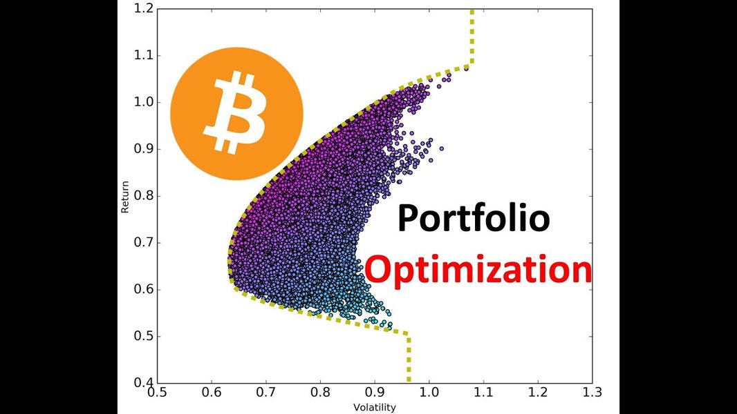
Visualizing portfolio optimization concepts often involves charts showing asset performance and allocation strategies.

The Reinforcement Learning Environment

To train our DDPG agent, we need a simulated environment that mimics the cryptocurrency market and portfolio management process. We create a custom environment class, often inheriting from `gym.Env` or following a similar interface.

Environment Components

• State Space: What the agent observes. This typically includes:
  • A lookback window of historical price changes or returns for all assets (e.g., the last 30 days).
  • The agent's current portfolio weights (allocation across cash/assets).
  This provides context about recent market trends and the agent's current position.
• Action Space: What the agent can do. This is a continuous vector of size 36, where each element represents the target weight for a cryptocurrency (e.g., values between -1 for short and +1 for long). Constraints (like sum of absolute weights <= 1 or 2 for leverage limits) are applied within the environment's step logic.
• Step Function (`step(action)`):
  1. Receives the agent's chosen action (target weights).
  2. Calculates the necessary trades to rebalance the portfolio from current weights to target weights.
  3. Applies transaction costs (e.g., a small percentage of the traded value).
  4. Calculates the portfolio value change based on the next day's price movements and the *new* weights.
  5. Determines the reward (often the change in portfolio value, potentially adjusted for risk).
  6. Calculates the next state based on the updated portfolio and market data.
  7. Returns the next state, reward, a 'done' flag (indicating the end of an episode/backtest), and optional info.
• Reset Function (`reset()`): Resets the environment to its initial state (start of the backtesting period, initial portfolio value, initial weights).

Deep Deterministic Policy Gradient (DDPG) Agent

The DDPG agent is the "brain" that learns the trading strategy. It consists of the Actor, Critic, their target counterparts, and a replay buffer.

Network Architectures

• Actor (`Actor` class): Typically a multi-layer perceptron (MLP) that takes the state as input and outputs the deterministic action (portfolio weights). The final layer often uses `tanh` activation to constrain the output between -1 and 1, which is then scaled if necessary.
• Critic (`Critic` class): Also usually an MLP. It takes both the state and the action (proposed by the actor or sampled from the buffer) as input and outputs a single Q-value, representing the expected cumulative reward.

Training Process

1. Initialize Actor, Critic, target networks, and replay buffer.
2. For each episode:
   • Reset the environment.
   • For each step:
     • Select an action using the Actor network + exploration noise.
     • Execute the action in the environment, observe reward and next state.
     • Store the transition (state, action, reward, next state, done) in the replay buffer.
     • Sample a batch of transitions from the replay buffer.
     • Update the Critic network by minimizing the MSE loss between the current Q-value and the target Q-value (calculated using the target networks).
     • Update the Actor network using the sampled policy gradient (aiming to maximize the Critic's output).
     • Perform soft updates on the target networks (slowly tracking the learned networks).

Agent Architecture Comparison

The radar chart below provides a conceptual comparison of DDPG against other potential RL approaches for this task based on common characteristics. Note that these are general tendencies and specific implementations can vary.

Key Hyperparameters and Setup

The performance of a DDPG agent is sensitive to hyperparameters. This table summarizes the specified parameters and typical network choices.

System Components Overview

This mind map illustrates the overall workflow and components involved in the DDPG crypto portfolio management system.

Python Implementation with PyTorch

Below is the Python code combining all the elements discussed. It includes data loading, ranking, the RL environment, the DDPG agent, training, and evaluation logic.

import pandas as pd
import numpy as np
import torch
import torch.nn as nn
import torch.optim as optim
import torch.nn.functional as F
import random
import matplotlib.pyplot as plt
from collections import deque
import os
import gym # Optional, for environment structure convention

# Ensure reproducibility (optional but recommended)
SEED = 42
torch.manual_seed(SEED)
np.random.seed(SEED)
random.seed(SEED)
# Set device
device = torch.device("cuda" if torch.cuda.is_available() else "cpu")
print(f"Using device: {device}")

# --- 1. Data Loading and Preprocessing ---
def load_and_preprocess_data(filepath='Mdata36.csv', rolling_window=30):
    """Loads data, calculates returns, volatility, Sharpe, and composite score."""
    try:
        df = pd.read_csv(filepath, parse_dates=['Date'], index_col='Date')
    except FileNotFoundError:
        print(f"Error: File not found at {filepath}")
        return None, None, None, None, None

    # Define the 36 crypto columns explicitly
    crypto_cols = ['ATOM', 'BAT', 'BNB', 'BTC', 'BUSD', 'DASH', 'DUSK', 'EOS', 'ETC',
                   'ETH', 'FET', 'ICX', 'LINK', 'LTC', 'MTL', 'NEO', 'NULS', 'OMG',
                   'ONE', 'ONG', 'ONT', 'PERL', 'QTUM', 'REN', 'RVN', 'THETA', 'TOMO',
                   'TRX', 'WAN', 'WAVES', 'XLM', 'XMR', 'XRP', 'XTZ', 'ZEC', 'ZRX']

    # Ensure only expected columns exist
    missing_cols = [col for col in crypto_cols if col not in df.columns]
    if missing_cols:
        print(f"Warning: The following columns are missing from the CSV: {missing_cols}")
        # Optionally filter df to only include available columns from crypto_cols
        crypto_cols = [col for col in crypto_cols if col in df.columns]

    df = df[crypto_cols]
    df = df.ffill().bfill() # Handle missing values

    # Calculate daily returns
    returns_df = df.pct_change().fillna(0) # Fill first row NaNs with 0

    # Calculate rolling volatility
    volatility_df = returns_df.rolling(window=rolling_window).std().fillna(0)

    # Calculate rolling mean return
    mean_return_df = returns_df.rolling(window=rolling_window).mean().fillna(0)

    # Calculate rolling Sharpe Ratio (assuming risk-free rate = 0)
    # Add small epsilon to denominator to avoid division by zero
    sharpe_df = mean_return_df / (volatility_df + 1e-9)
    sharpe_df = sharpe_df.replace([np.inf, -np.inf], 0).fillna(0)

    # --- Composite Score Calculation (Rank Averaging) ---
    # Rank based on Sharpe (higher is better)
    sharpe_ranks = sharpe_df.rank(axis=1, ascending=False, method='first')
    # Rank based on recent mean return (higher is better)
    return_ranks = mean_return_df.rank(axis=1, ascending=False, method='first')
    # Rank based on volatility (lower is better)
    volatility_ranks = volatility_df.rank(axis=1, ascending=True, method='first')

    # Average the ranks: Lower average rank is better
    composite_ranks = (sharpe_ranks + return_ranks + volatility_ranks) / 3
    # Final ranking: Rank the average ranks (ascending, so rank 1 is the best)
    daily_final_ranks = composite_ranks.rank(axis=1, ascending=True, method='first')

    print(f"Data loaded and processed. Shape: {df.shape}")
    print(f"Returns calculated. Shape: {returns_df.shape}")
    print(f"Volatility calculated. Shape: {volatility_df.shape}")
    print(f"Sharpe calculated. Shape: {sharpe_df.shape}")
    print(f"Daily Ranks calculated. Shape: {daily_final_ranks.shape}")

    # Align dataframes - start after the initial rolling window period
    start_index = df.index[rolling_window - 1]
    prices_df_aligned = df.loc[start_index:]
    returns_df_aligned = returns_df.loc[start_index:]
    daily_final_ranks_aligned = daily_final_ranks.loc[start_index:]

    return prices_df_aligned, returns_df_aligned, daily_final_ranks_aligned, crypto_cols

def plot_ranking(daily_ranks_df, num_assets_to_plot=5, title="Crypto Ranking Evolution"):
    """Plots the daily ranking evolution for a specified number of assets."""
    plt.figure(figsize=(15, 7))
    assets_to_plot = daily_ranks_df.columns[:num_assets_to_plot]
    for asset in assets_to_plot:
        plt.plot(daily_ranks_df.index, daily_ranks_df[asset], label=asset)

    plt.title(title)
    plt.xlabel("Date")
    plt.ylabel("Rank (1 = Best)")
    plt.gca().invert_yaxis() # Show rank 1 at the top
    plt.legend()
    plt.grid(True)
    plt.tight_layout()
    plt.show()

# --- 2. Reinforcement Learning Environment ---
class CryptoPortfolioEnv:
    """Custom environment for crypto portfolio management."""
    def __init__(self, prices_df, returns_df, initial_balance=10000, lookback_window=30, trading_cost_bps=10):
        self.prices_df = prices_df
        self.returns_df = returns_df
        self.dates = prices_df.index
        self.crypto_cols = prices_df.columns.tolist()
        self.n_assets = len(self.crypto_cols)

        self.initial_balance = initial_balance
        self.lookback_window = lookback_window
        self.trading_cost_rate = trading_cost_bps / 10000.0 # Basis points to rate

        # State space: [lookback returns] + [current weights]
        self.state_dim = self.n_assets * self.lookback_window + self.n_assets

        # Action space: target weights for each asset [-1, 1]
        self.action_dim = self.n_assets
        self.max_action = 1.0

        # Initialize state variables
        self.current_step = 0
        self.balance = 0.0
        self.portfolio_value = 0.0
        self.weights = np.zeros(self.n_assets) # Current weights

        self.history = [] # For tracking portfolio value

    def reset(self):
        """Resets the environment to the beginning of the data."""
        self.current_step = self.lookback_window # Start after initial lookback period
        self.balance = self.initial_balance # Assume all cash initially
        self.weights = np.zeros(self.n_assets) # No assets held initially
        self.portfolio_value = self.initial_balance
        self.history = [(self.dates[self.current_step-1], self.portfolio_value)]
        return self._get_state()

    def _get_state(self):
        """Returns the current state representation."""
        if self.current_step < self.lookback_window:
             # Should not happen if reset correctly, but handle defensively
             return np.zeros(self.state_dim)

        # Get returns for the lookback window ending at the *previous* step
        start_idx = self.current_step - self.lookback_window
        end_idx = self.current_step
        lookback_returns = self.returns_df.iloc[start_idx:end_idx].values.flatten()

        # Concatenate lookback returns and current weights
        state = np.concatenate([lookback_returns, self.weights])
        return state

    def step(self, action):
        """Takes an action (target weights) and steps the environment forward."""
        # Ensure action is numpy array
        action = np.asarray(action)

        # Clip action to bounds [-max_action, max_action]
        target_weights = np.clip(action, -self.max_action, self.max_action)

        # --- Apply Leverage Constraint (Optional but recommended for long-short) ---
        # Example: Max leverage of 1 (sum of absolute weights <= 1)
        leverage_limit = 1.0
        current_abs_sum = np.sum(np.abs(target_weights))
        if current_abs_sum > leverage_limit:
            target_weights = target_weights * (leverage_limit / current_abs_sum)

        # --- Rebalancing Calculation ---
        # Get prices for the *current* day (end of the previous step)
        current_prices = self.prices_df.iloc[self.current_step - 1].values

        # Calculate current portfolio value *before* rebalancing
        # Note: This assumes 'balance' represents cash, and value comes from assets.
        # A more robust model might track units of each asset.
        # For simplicity here, assume weights represent fraction of *total value*.
        current_portfolio_value = self.portfolio_value

        # Calculate value of current holdings for each asset
        current_asset_values = self.weights * current_portfolio_value

        # Calculate target value for each asset based on target weights
        target_asset_values = target_weights * current_portfolio_value

        # Calculate the value of trades needed (positive = buy, negative = sell)
        trade_values = target_asset_values - current_asset_values

        # Calculate total transaction cost
        total_trading_cost = np.sum(np.abs(trade_values)) * self.trading_cost_rate

        # --- Update Portfolio Value for the *Next* Day ---
        # Get returns for the *current* day (which affect the value at the start of the *next* step)
        today_returns = self.returns_df.iloc[self.current_step].values

        # Calculate portfolio return based on the *target* weights (post-rebalancing)
        # R_portfolio = sum(w_i * R_i)
        portfolio_return_gross = np.sum(target_weights * today_returns)

        # Update portfolio value: Value_t+1 = Value_t * (1 + R_portfolio_gross) - TradingCost
        self.portfolio_value = current_portfolio_value * (1 + portfolio_return_gross) - total_trading_cost

        # Ensure portfolio value doesn't go below zero (ruin)
        self.portfolio_value = max(self.portfolio_value, 0)

        # Update weights to the target weights for the next state calculation
        self.weights = target_weights

        # Calculate reward: Change in portfolio value is a common choice
        # Alternatively, use log return or risk-adjusted return
        reward = self.portfolio_value - current_portfolio_value
        # reward = np.log(self.portfolio_value / current_portfolio_value) if current_portfolio_value > 1e-9 else 0


        # Move to the next day
        self.current_step += 1

        # Check if done (reached end of data)
        done = self.current_step >= len(self.prices_df)

        # Get the next state
        next_state = self._get_state() if not done else np.zeros(self.state_dim)

        # Store history
        if not done:
           self.history.append((self.dates[self.current_step-1], self.portfolio_value))
        else:
           # If done, record final value with last valid date
           self.history.append((self.dates[-1], self.portfolio_value))


        return next_state, reward, done, {"portfolio_value": self.portfolio_value}

# --- 3. DDPG Agent Implementation ---

# Ornstein-Uhlenbeck Noise (Common exploration noise for DDPG)
class OUNoise:
    def __init__(self, size, seed, mu=0., theta=0.15, sigma=0.2):
        self.mu = mu * np.ones(size)
        self.theta = theta
        self.sigma = sigma
        self.seed = random.seed(seed)
        self.size = size
        self.reset()

    def reset(self):
        self.state = np.copy(self.mu)

    def sample(self):
        x = self.state
        dx = self.theta * (self.mu - x) + self.sigma * np.random.randn(self.size)
        self.state = x + dx
        return self.state

# Actor Network
class Actor(nn.Module):
    def __init__(self, state_dim, action_dim, max_action):
        super(Actor, self).__init__()
        self.fc1 = nn.Linear(state_dim, 256)
        self.fc2 = nn.Linear(256, 256)
        self.fc3 = nn.Linear(256, action_dim)
        self.max_action = max_action

    def forward(self, state):
        x = F.relu(self.fc1(state))
        x = F.relu(self.fc2(x))
        # Use tanh to output actions between -1 and 1, then scale
        action = self.max_action * torch.tanh(self.fc3(x))
        return action

# Critic Network
class Critic(nn.Module):
    def __init__(self, state_dim, action_dim):
        super(Critic, self).__init__()
        # Layer 1
        self.fc1_state = nn.Linear(state_dim, 128)
        self.fc1_action = nn.Linear(action_dim, 128)
        # Layer 2
        self.fc2 = nn.Linear(256, 256) # Combined state-action path
        # Layer 3
        self.fc3 = nn.Linear(256, 1) # Output Q-value

    def forward(self, state, action):
        s1 = F.relu(self.fc1_state(state))
        a1 = F.relu(self.fc1_action(action))
        x = torch.cat((s1, a1), dim=1)
        x = F.relu(self.fc2(x))
        q_value = self.fc3(x)
        return q_value

# Replay Buffer
class ReplayBuffer:
    def __init__(self, capacity):
        self.capacity = capacity
        self.buffer = deque(maxlen=capacity)

    def push(self, state, action, reward, next_state, done):
        self.buffer.append((state, action, reward, next_state, float(done))) # Ensure done is float

    def sample(self, batch_size):
        batch = random.sample(self.buffer, batch_size)
        state, action, reward, next_state, done = map(np.stack, zip(*batch))
        return state, action, reward, next_state, done

    def __len__(self):
        return len(self.buffer)

# DDPG Agent Class
class DDPGAgent:
    def __init__(self, state_dim, action_dim, max_action, lr_actor=3e-4, lr_critic=3e-4, discount=0.99, tau=0.005, buffer_capacity=100000):
        self.actor = Actor(state_dim, action_dim, max_action).to(device)
        self.actor_target = Actor(state_dim, action_dim, max_action).to(device)
        self.actor_target.load_state_dict(self.actor.state_dict())
        self.actor_optimizer = optim.Adam(self.actor.parameters(), lr=lr_actor)

        self.critic = Critic(state_dim, action_dim).to(device)
        self.critic_target = Critic(state_dim, action_dim).to(device)
        self.critic_target.load_state_dict(self.critic.state_dict())
        self.critic_optimizer = optim.Adam(self.critic.parameters(), lr=lr_critic)

        self.replay_buffer = ReplayBuffer(buffer_capacity)
        self.noise = OUNoise(action_dim, seed=SEED) # Exploration noise

        self.discount = discount
        self.tau = tau
        self.max_action = max_action

    def select_action(self, state, add_noise=True):
        state = torch.FloatTensor(state.reshape(1, -1)).to(device)
        self.actor.eval() # Set actor to evaluation mode
        with torch.no_grad():
            action = self.actor(state).cpu().data.numpy().flatten()
        self.actor.train() # Set actor back to train mode

        if add_noise:
            noise = self.noise.sample()
            action = action + noise

        # Clip action to ensure it's within valid bounds
        return np.clip(action, -self.max_action, self.max_action)

    def train(self, batch_size):
        if len(self.replay_buffer) < batch_size:
            return # Not enough samples yet

        # Sample a batch from the replay buffer
        state, action, reward, next_state, done = self.replay_buffer.sample(batch_size)

        # Convert batch to tensors
        state = torch.FloatTensor(state).to(device)
        action = torch.FloatTensor(action).to(device)
        reward = torch.FloatTensor(reward).unsqueeze(1).to(device)
        next_state = torch.FloatTensor(next_state).to(device)
        done = torch.FloatTensor(done).unsqueeze(1).to(device)

        # --- Critic Update ---
        with torch.no_grad():
            # Select next action according to target actor:
            next_action = self.actor_target(next_state)
            # Compute the target Q value:
            target_Q = self.critic_target(next_state, next_action)
            target_Q = reward + ((1 - done) * self.discount * target_Q)

        # Get current Q estimate:
        current_Q = self.critic(state, action)

        # Compute critic loss:
        critic_loss = F.mse_loss(current_Q, target_Q)

        # Optimize the critic:
        self.critic_optimizer.zero_grad()
        critic_loss.backward()
        # torch.nn.utils.clip_grad_norm_(self.critic.parameters(), 1.0) # Optional: Gradient clipping
        self.critic_optimizer.step()

        # --- Actor Update ---
        # Compute actor loss (policy gradient):
        actor_actions = self.actor(state)
        actor_loss = -self.critic(state, actor_actions).mean() # Maximize Q-value

        # Optimize the actor:
        self.actor_optimizer.zero_grad()
        actor_loss.backward()
        # torch.nn.utils.clip_grad_norm_(self.actor.parameters(), 1.0) # Optional: Gradient clipping
        self.actor_optimizer.step()

        # --- Soft Update Target Networks ---
        for param, target_param in zip(self.critic.parameters(), self.critic_target.parameters()):
            target_param.data.copy_(self.tau * param.data + (1 - self.tau) * target_param.data)

        for param, target_param in zip(self.actor.parameters(), self.actor_target.parameters()):
            target_param.data.copy_(self.tau * param.data + (1 - self.tau) * target_param.data)

    def save(self, filename):
        torch.save(self.critic.state_dict(), filename + "_critic.pth")
        torch.save(self.critic_optimizer.state_dict(), filename + "_critic_optimizer.pth")
        torch.save(self.actor.state_dict(), filename + "_actor.pth")
        torch.save(self.actor_optimizer.state_dict(), filename + "_actor_optimizer.pth")

    def load(self, filename):
        self.critic.load_state_dict(torch.load(filename + "_critic.pth", map_location=device))
        self.critic_optimizer.load_state_dict(torch.load(filename + "_critic_optimizer.pth", map_location=device))
        self.critic_target.load_state_dict(self.critic.state_dict()) # Load critic weights into target

        self.actor.load_state_dict(torch.load(filename + "_actor.pth", map_location=device))
        self.actor_optimizer.load_state_dict(torch.load(filename + "_actor_optimizer.pth", map_location=device))
        self.actor_target.load_state_dict(self.actor.state_dict()) # Load actor weights into target


# --- 4. Training and Evaluation ---

def run_experiment(prices_df, returns_df, num_episodes=50, batch_size=64, lookback_window=30):
    """Runs the training and evaluation process."""

    # Data Splitting (70% train, 30% validation)
    split_index = int(len(prices_df) * 0.7)
    train_prices = prices_df.iloc[:split_index]
    train_returns = returns_df.iloc[:split_index]
    val_prices = prices_df.iloc[split_index:]
    val_returns = returns_df.iloc[split_index:]

    print(f"Training data range: {train_prices.index.min()} to {train_prices.index.max()}")
    print(f"Validation data range: {val_prices.index.min()} to {val_prices.index.max()}")

    # Create Environments
    train_env = CryptoPortfolioEnv(train_prices, train_returns, lookback_window=lookback_window)
    val_env = CryptoPortfolioEnv(val_prices, val_returns, lookback_window=lookback_window)

    # Initialize Agent
    state_dim = train_env.state_dim
    action_dim = train_env.action_dim
    max_action = train_env.max_action
    agent = DDPGAgent(state_dim, action_dim, max_action, discount=0.99, lr_actor=3e-4, lr_critic=3e-4)

    # --- Training Loop ---
    print("\n--- Starting Training ---")
    training_portfolio_values = []
    for episode in range(num_episodes):
        state = train_env.reset()
        agent.noise.reset() # Reset noise process
        episode_reward = 0
        done = False
        step = 0

        while not done:
            action = agent.select_action(state, add_noise=True)
            next_state, reward, done, info = train_env.step(action)
            agent.replay_buffer.push(state, action, reward, next_state, done)
            state = next_state
            episode_reward += reward
            step += 1

            # Train the agent periodically
            if len(agent.replay_buffer) > batch_size:
                 agent.train(batch_size)

            if done:
                final_value = info['portfolio_value']
                training_portfolio_values.append(final_value)
                print(f"Episode {episode+1}/{num_episodes}, Steps: {step}, Final Value: {final_value:.2f}, Total Reward: {episode_reward:.2f}")

    # Save the trained agent
    agent.save("ddpg_crypto_agent")
    print("Training finished and agent saved.")

    # --- Evaluation ---
    print("\n--- Starting Evaluation ---")
    state = val_env.reset()
    done = False
    while not done:
        action = agent.select_action(state, add_noise=False) # No noise during evaluation
        next_state, reward, done, info = val_env.step(action)
        state = next_state
        if done:
            print(f"Evaluation Final Portfolio Value: {info['portfolio_value']:.2f}")

    # --- Plot Results ---
    # Plot Training Episode Values
    plt.figure(figsize=(12, 6))
    plt.plot(range(1, num_episodes + 1), training_portfolio_values, marker='o', linestyle='-')
    plt.xlabel("Episode")
    plt.ylabel("Final Portfolio Value")
    plt.title("Portfolio Value at End of Each Training Episode")
    plt.grid(True)
    plt.tight_layout()
    plt.show()

    # Plot Evaluation Portfolio History
    eval_history_df = pd.DataFrame(val_env.history, columns=['Date', 'PortfolioValue'])
    eval_history_df.set_index('Date', inplace=True)

    plt.figure(figsize=(12, 6))
    plt.plot(eval_history_df.index, eval_history_df['PortfolioValue'])
    plt.xlabel("Date")
    plt.ylabel("Portfolio Value")
    plt.title("Portfolio Value During Validation Period")
    plt.grid(True)
    plt.tight_layout()
    plt.show()


# --- Main Execution ---
if __name__ == "__main__":
    FILEPATH = 'Mdata36.csv'
    ROLLING_WINDOW = 30
    LOOKBACK_WINDOW = 30 # Must be >= ROLLING_WINDOW
    NUM_EPISODES = 20 # Increase for real training (e.g., 100+)
    BATCH_SIZE = 128

    prices_df, returns_df, daily_ranks_df, crypto_cols = load_and_preprocess_data(FILEPATH, ROLLING_WINDOW)

    if prices_df is not None:
        # Plot initial ranking
        plot_ranking(daily_ranks_df, num_assets_to_plot=5)

        # Run training and evaluation
        run_experiment(prices_df, returns_df,
                       num_episodes=NUM_EPISODES,
                       batch_size=BATCH_SIZE,
                       lookback_window=LOOKBACK_WINDOW)
    else:
        print("Could not proceed due to data loading issues.")

  

Code Explanation

• Data Handling: `load_and_preprocess_data` loads the CSV, computes returns, rolling metrics (volatility, Sharpe), and derives daily ranks using rank averaging. It handles missing data and aligns the dataframes. `plot_ranking` visualizes the ranks.
• Environment (`CryptoPortfolioEnv`): Simulates the trading process. The `step` function handles action application, leverage constraints, rebalancing costs, portfolio value updates based on daily returns, and reward calculation. The state includes lookback returns and current weights.
• DDPG Agent (`DDPGAgent`): Contains the Actor, Critic, target networks, and replay buffer. `select_action` chooses weights (with optional noise), and `train` performs the DDPG updates using sampled batches. OUNoise is used for exploration. `save`/`load` methods are included.
• Training/Evaluation (`run_experiment`): Splits data, creates environments, initializes the agent, runs the training loop (saving the agent), performs evaluation on the validation set, and plots the results (end-of-episode training values and validation portfolio history).
• Main Block: Sets parameters, calls the data loading/plotting functions, and executes the `run_experiment` function.

Note on Entropy Regularization: The request mentioned entropy regularization. Standard DDPG uses action noise (like the implemented OUNoise) for exploration. Algorithms like Soft Actor-Critic (SAC) explicitly incorporate an entropy term in the objective function to encourage exploration by maximizing policy entropy alongside reward. Implementing true entropy regularization in DDPG typically requires modifying the actor to output parameters of a probability distribution (making it stochastic) and adding an entropy bonus to the actor's loss, which deviates from the standard DDPG algorithm structure presented here.

Training and Evaluation Insights

The training process involves the agent interacting with the training data over multiple episodes. In each episode, it starts with an initial balance and tries to maximize its final portfolio value by learning optimal allocation weights. The `run_experiment` function shows the final portfolio value at the end of each training episode, which should ideally trend upwards as the agent learns.

The evaluation phase tests the trained agent (without exploration noise) on the unseen validation data (the final 30%). This provides a more realistic estimate of how the learned strategy might perform in the future. The plot of the portfolio value during validation shows the agent's performance on this out-of-sample data.

Key aspects to monitor:

• Convergence: Does the portfolio value during training stabilize or consistently improve?
• Generalization: How does the performance on the validation set compare to the training set? Significant drops might indicate overfitting.
• Risk vs. Reward: While this implementation primarily uses portfolio value change as reward, analyzing the volatility or drawdown of the portfolio during validation is crucial for assessing risk.
• Hyperparameter Impact: Performance is sensitive to learning rates, discount factor, noise parameters, network sizes, and buffer/batch sizes. Experimentation is often needed.

Understanding DDPG Exploration in Action

DDPG's ability to handle continuous action spaces makes it suitable for tasks like portfolio allocation. The video below provides a conceptual overview and implementation details for DDPG, illustrating how Actor-Critic methods work in continuous environments.

Frequently Asked Questions (FAQ)

References

• Quantitative Trading with Deep Deterministic Policy Gradients (DDPG) - Medium
• pytorch-deeprl-DDPG-EIIE.ipynb - GitHub
• pytorch-ddpg implementation - GitHub
• PyTorch-DDPG-Stock-Trading - GitHub
• A Practical Guide for Portfolio Management with Deep Reinforcement Learning in Crypto Market - arXiv
• Cryptocurrency Risk-Adjusted Returns: Sharpe Ratios - CryptoDataDownload
• Deep Deterministic Policy Gradient (DDPG) Agent for Portfolio Management: An Example - Medium

Recommended Further Exploration

How does Soft Actor-Critic (SAC) compare to DDPG for crypto trading?

Can incorporating technical indicators improve the DDPG agent's performance?

How to implement risk management rules like stop-loss or max drawdown limits in the RL environment?

What are the effects of different reward functions (e.g., Sharpe ratio vs. profit) on the learned trading strategy?

ui.adsabs.harvard.edu

Deep Reinforcement Learning for Long-Short Portfolio Optimization

github.com

GitHub - schneimo/ddpg-pytorch: PyTorch implementation of DDPG for continuous control tasks.

themerkle.com

Sharpe Ratio Signal Highlights Risk-Adjusted Performance of Key Crypto ...

sciencedirect.com

A novel Deep Reinforcement Learning based automated stock ...

github.com

GitHub - JoshuaWu1997/PyTorch-DDPG-Stock-Trading: An implementation of DDPG using PyTorch for algorithmic trading on Chinese SH50 stock market.

medium.com

Deep Deterministic Policy Gradient (DDPG) Agent for Portfolio ...

charts.bitbo.io

Bitcoin Sharpe Ratio

reddit.com

Clear and Concise DDPG and TD3 Implementations in PyTorch

medium.com

Crypto price predictions with PyTorch and TensorFlow | by Deephaven Data Labs | Medium

pytorch.org

Competitive Multi-Agent Reinforcement Learning (DDPG ... - PyTorch

medium.com

Quantitative Trading with Deep Deterministic Policy Gradients(DDPG) | by Renjie Ge | Medium

reddit.com

Does it make sense to use RL for trading? : r/reinforcementlearning

researchgate.net

deep reinforcement learning for investment portfolio rebalancing

reddit.com

Updated Bitcoin Vs. S&P Total Return Sharpe Ratios - Reddit

medium.com

Deep Reinforcement Learning for Crypto Trading | by Alex K - Medium

github.com

rl-portfolio-management/pytorch-deeprl-DDPG-EIIE.ipynb at master · wassname/rl-portfolio-management

medium.com

Trading Through Reinforcement Learning using LSTM Neural Networks ...

arxiv.org

[2503.09655] A Deep Reinforcement Learning Approach to Automated ...

binance.com

Sharpe Ratio: The Key Metric Every Cryptocurrency Investor Needs ...

neptune.ai

7 Applications of Reinforcement Learning in Finance and Trading

medium.com

Using Reinforcement Learning to Optimize Stock Trading Strategies ...

sciencedirect.com

Performance measurement of crypto funds - ScienceDirect

cognizium.io

[PDF] Cryptocurrencies and the Sharpe Ratio of Traditional Investment ...

fidelitydigitalassets.com

A Closer Look at Bitcoin's Volatility - Fidelity Digital Assets

blog.mlq.ai

Deep Reinforcement Learning for Trading: Strategy Development & AutoML

github.com

GitHub - XinJingHao/DDPG-Pytorch: A clean Pytorch implementation of DDPG on continuous action space.

newhedge.io

Bitcoin Sharpe Ratio Chart - Newhedge

cs229.stanford.edu

[PDF] Stock Trading with Recurrent Reinforcement Learning (RRL) - CS229

blog.quantinsti.com

Reinforcement Learning in Trading: Components, Challenges, and More

cryptodatadownload.com

Major Cryptocurrency Risk Adjusted Return Comparisons with Sharpe Ratios

zhuanlan.zhihu.com

FinRL Ecosystem Tutorial and Introduction (Part II) - 知乎专栏

twosigma.com

Risk Analysis of Crypto Assets - Two Sigma

diposit.ub.edu

[PDF] AutoTrading with Reinforcement Learning

statista.com

Bitcoin return on investment 2024| Statista - Sharpe ratio

arxiv.org

[2106.08437] Deep reinforcement learning on a multi-asset environment ...

arxiv.org

[PDF] Deep Reinforcement Learning for Long-Short Portfolio Optimization

medium.com

Cryptocurrencies & The Sharpe Ratio | by Ciaran Mcveigh - Medium

recipp.ipp.pt

[PDF] Portfolio Allocation using Deep Reinforcement Learning

medium.com

DEEP REINFORCEMENT LEARNING IN ALGORITHMIC TRADING (Part- II) | ...

arxiv.org

Reinforcement Learning Framework for Quantitative Trading

alphaarchitect.com

Deep Reinforcement Learning for trading applications

arxiv.org

Portfolio Management using Deep Reinforcement Learning

paperswithcode.com

Cryptocurrency Portfolio Management with Deep Reinforcement ...

medium.com

Deep Reinforcement Learning for Crypto Trading | by Alex K - Medium

github.com

GitHub - ghliu/pytorch-ddpg: Implementation of the Deep Deterministic Policy Gradient (DDPG) using PyTorch

portfolioslab.com

Crypto Portfolio | PortfoliosLab

github.com

GitHub - adi3e08/DDPG: A clean and minimal implementation of DDPG (Deep Deterministic Policy Gradient) algorithm in Pytorch.