
Unlocking the Quantum Realm: How Qubits Are Revolutionizing Computation
A technical dive into the strange and powerful world of quantum computing principles, models, programming, and algorithms.
Quantum computing represents a fundamental shift in how we process information, moving beyond the binary limits of classical computers. By harnessing the counterintuitive principles of quantum mechanics, this emerging field promises to tackle problems currently intractable for even the most powerful supercomputers. This introduction provides a technical overview for learners, covering the core concepts, computational models, programming paradigms, and illustrative algorithms that define quantum computing.
Highlights: Core Quantum Concepts
- Qubits, Superposition, and Entanglement: Unlike classical bits (0 or 1), quantum bits (qubits) can exist in multiple states simultaneously (superposition) and can be intrinsically linked (entangled), enabling massive parallel processing capabilities.
- Quantum Circuit Model: This is the standard framework for designing quantum algorithms and analyzing their complexity, analogous to classical circuit models but using quantum gates acting on qubits.
- Potential for Exponential Speedup: For specific types of problems, such as factoring large numbers or simulating quantum systems, quantum algorithms offer the potential for dramatic, often exponential, speedups over the best known classical algorithms.
Foundations of Quantum Computation
Understanding quantum computing requires grasping several key concepts derived directly from quantum mechanics. These principles differentiate quantum computation from its classical counterpart.
Quantum Bits (Qubits)
The fundamental unit of quantum information is the qubit. While a classical bit is restricted to being either a 0 or a 1, a qubit can exist in a state of superposition, representing a combination of both 0 and 1 simultaneously. Mathematically, the state of a single qubit, denoted as \(|\psi\rangle\), is described as a linear combination of its basis states, \(|0\rangle\) and \(|1\rangle\):
\[ |\psi\rangle = \alpha|0\rangle + \beta|1\rangle \]Here, \(\alpha\) and \(\beta\) are complex numbers called probability amplitudes. The squares of their magnitudes, \(|\alpha|^2\) and \(|\beta|^2\), represent the probabilities of the qubit collapsing to the state \(|0\rangle\) or \(|1\rangle\) respectively, upon measurement. These probabilities must sum to 1: \(|\alpha|^2 + |\beta|^2 = 1\).
This ability to exist in multiple states at once allows a system of \(n\) qubits to represent \(2^n\) states simultaneously, offering an exponential increase in information capacity compared to \(n\) classical bits.
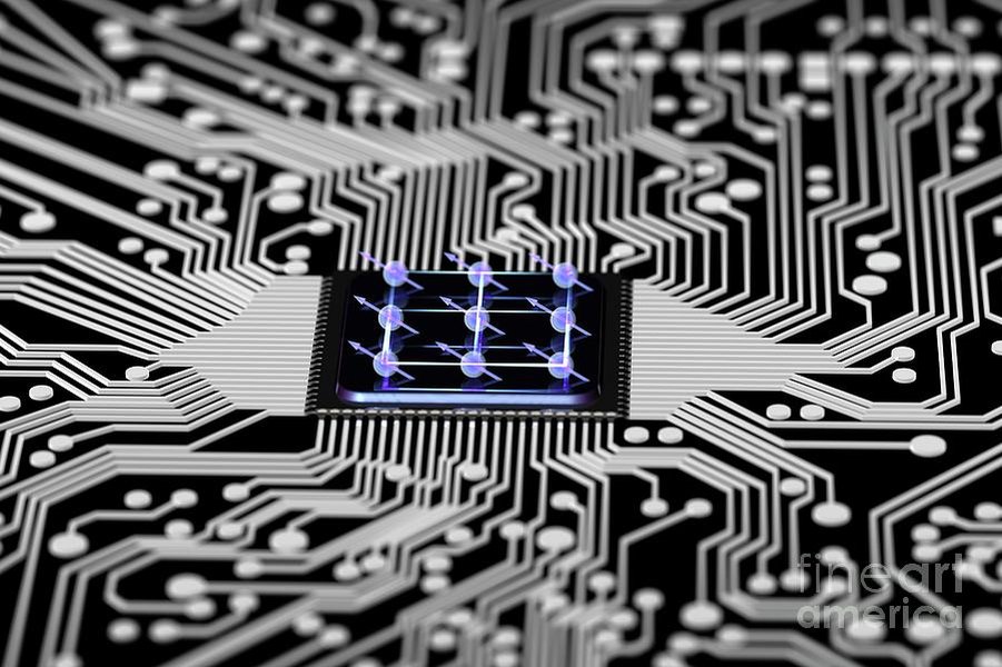
Conceptual representation of qubits and quantum operations.
Entanglement
Entanglement is perhaps one of the most non-intuitive aspects of quantum mechanics. It describes a strong correlation between two or more qubits. When qubits are entangled, their fates are linked, regardless of the physical distance separating them. Measuring the state of one entangled qubit instantaneously influences the state of the other(s). For example, in the entangled Bell state \(\frac{|00\rangle + |11\rangle}{\sqrt{2}}\), if the first qubit is measured to be 0, the second qubit will instantly be found to be 0 as well, and vice versa for the state 1. Entanglement is a crucial resource in many quantum algorithms and communication protocols.
Quantum Gates and Circuits
Similar to classical logic gates (like AND, OR, NOT) operating on bits, quantum gates perform operations on qubits. These gates are represented by unitary matrices, ensuring that the operations are reversible (except for measurement). Common examples include:
- Pauli Gates (X, Y, Z): The Pauli-X gate is analogous to a classical NOT gate, flipping \(|0\rangle\) to \(|1\rangle\) and vice versa.
- Hadamard Gate (H): This crucial gate creates superposition, transforming \(|0\rangle\) into \(\frac{|0\rangle + |1\rangle}{\sqrt{2}}\) and \(|1\rangle\) into \(\frac{|0\rangle - |1\rangle}{\sqrt{2}}\).
- Controlled-NOT Gate (CNOT): A two-qubit gate essential for creating entanglement. It flips the target qubit if and only if the control qubit is in the state \(|1\rangle\).
A quantum circuit is a sequence of these quantum gates applied to a set of qubits, typically followed by a measurement step to extract a classical result. The design of these circuits forms the basis of quantum algorithm development.
Measurement
Quantum computation culminates in measurement, the process of observing the state of the qubits. Measurement is inherently probabilistic and causes the qubit's superposition to collapse into one of the definite classical states (0 or 1), with probabilities determined by the squared amplitudes (\(|\alpha|^2\) or \(|\beta|^2\)). Due to this probabilistic nature, quantum algorithms are often run multiple times to determine the most likely outcome.
Decoherence and Error Correction
Quantum states are extremely fragile and susceptible to environmental noise (e.g., temperature fluctuations, electromagnetic fields), which can cause them to lose their quantum properties – a process called decoherence. This leads to errors in computation. Significant research efforts are focused on developing quantum error correction codes and building fault-tolerant quantum hardware to mitigate these effects. Current quantum computers operate in the "Noisy Intermediate-Scale Quantum" (NISQ) era, where noise limits the complexity and duration of computations.

Conceptual depiction related to managing errors in quantum systems.
Visualizing Quantum Concepts
To better understand the core ideas and their interrelations, the following mindmap provides a visual overview of the foundational concepts in quantum computing.
(\(\alpha|0\rangle + \beta|1\rangle\))"] id1_1_2["Measurement
(Probabilistic Collapse)"] id1_2["Entanglement"] id1_2_1["Non-local Correlation"] id1_2_2["Resource for Algorithms"] id1_3["Quantum Gates"] id1_3_1["Unitary Operations"] id1_3_2["Examples: H, CNOT, Pauli-X"] id1_4["Quantum Circuits"] id1_4_1["Sequence of Gates"] id1_4_2["Algorithm Implementation"] id2["Computational Model"] id2_1["Quantum Circuit Model"] id2_1_1["Complexity Analysis (BQP)"] id2_1_2["Universality"] id2_2["Other Models
(Adiabatic, Topological)"] id3["Programming & Algorithms"] id3_1["Algorithm Design"] id3_1_1["Exploiting Quantum Phenomena"] id3_1_2["Reversibility"] id3_1_3["No-Cloning Theorem"] id3_2["Implementation"] id3_2_1["Quantum SDKs (Qiskit, Q#)"] id3_2_2["Simulation & Hardware Execution"] id3_3["Example Algorithms"] id3_3_1["Deutsch's Algorithm"] id3_3_2["Grover's Algorithm"] id3_3_3["Shor's Algorithm"] id4["Challenges & Applications"] id4_1["Decoherence & Noise"] id4_1_1["Error Correction"] id4_1_2["Fault Tolerance"] id4_2["Hardware Development"] id4_2_1["NISQ Era"] id4_2_2["Scaling Qubits"] id4_3["Potential Applications"] id4_3_1["Cryptography"] id4_3_2["Drug Discovery"] id4_3_3["Material Science"] id4_3_4["Optimization"] id4_3_5["Machine Learning"]
This mindmap illustrates how qubits, superposition, and entanglement form the basis for quantum gates and circuits, which are analyzed using computational models and used to design algorithms, while acknowledging the challenges and potential applications of the field.
Quantum vs. Classical Computation: A Comparative Look
While quantum computers offer potential advantages, they are not universally superior to classical computers. Their strengths lie in specific types of problems where quantum phenomena can be effectively leveraged. The radar chart below provides a conceptual comparison across several dimensions.
This chart highlights that while quantum computers excel in areas like quantum simulation, factorization, and potentially search, classical computers remain dominant for general tasks, have much lower error rates currently, and are far more accessible and mature. Note that the values are conceptual representations of relative strengths and weaknesses.
Modeling Quantum Computation for Complexity Analysis
To rigorously analyze the efficiency of quantum algorithms and compare their power to classical algorithms, a formal model of computation is needed. The most widely accepted and suitable model for this purpose is the Quantum Circuit Model.
The Quantum Circuit Model
Analogous to classical Boolean circuits, the quantum circuit model represents a computation as a sequence of quantum gates applied to an initial state of qubits (usually all \(|0\rangle\)). The circuit diagram flows from left to right, with horizontal lines representing qubits and boxes representing quantum gates acting on them. The computation concludes with measurements performed on some or all qubits to yield classical output.
Key Features for Complexity Analysis:
- Universality: A finite set of quantum gates (e.g., Hadamard, Phase, CNOT, and T gates) is sufficient to approximate any unitary operation, meaning the model is universal for quantum computation.
- Resource Measurement: Computational complexity is measured primarily by:
- Time Complexity: The number of gates in the circuit (or more accurately, the circuit depth – the number of time steps required).
- Space Complexity: The number of qubits required.
- Complexity Classes: This model allows the definition of quantum complexity classes. The most important is BQP (Bounded-Error Quantum Polynomial time), which contains decision problems solvable by a quantum computer in polynomial time with an error probability of at most 1/3. Problems like integer factorization (solved by Shor's algorithm) are known to be in BQP but are not believed to be in P (classical polynomial time).
The quantum circuit model provides a concrete framework for algorithm designers to specify computations and for theorists to analyze their resource requirements and compare them against classical complexity classes.
Programming a Quantum Computer: An Algorithm Designer's Viewpoint
Programming a quantum computer is fundamentally different from classical programming. It requires thinking in terms of manipulating quantum states (amplitudes and phases) rather than definite binary values.
The Design Process
From an algorithm designer's perspective, the process typically involves:
- Problem Mapping: Translating a computational problem into a form suitable for quantum computation. This often involves encoding input data into the initial state of qubits.
- Algorithm Construction: Designing a sequence of quantum gates (a quantum circuit) that evolves the initial state of the qubits. The goal is to manipulate the quantum state such that the amplitudes corresponding to the desired solution(s) are amplified, while others are diminished through quantum interference.
- Leveraging Quantum Phenomena: Actively utilizing superposition to explore multiple possibilities simultaneously and entanglement to create correlations needed for complex operations or speedups.
- Measurement Strategy: Determining which qubits to measure and how to interpret the probabilistic outcomes. Since measurement collapses the state, algorithms must be designed so that measuring yields the correct answer with high probability. Multiple runs are usually needed.
- Dealing with Constraints:
- Noise and Decoherence: Current hardware is noisy. Designers must consider the impact of errors and potentially use error mitigation techniques or design algorithms robust to noise. Quantum error correction codes are essential for future fault-tolerant machines but add significant overhead.
- No-Cloning Theorem: An unknown quantum state cannot be perfectly copied. This constraint influences how information is processed and duplicated within an algorithm.
- Hardware Limitations: Limited qubit counts, connectivity between qubits, and gate fidelities on current devices restrict the size and complexity of algorithms that can be run.
- Simulation and Execution: Using classical simulators to test and debug the algorithm's logic. Once validated, the algorithm can be run on actual quantum hardware using cloud platforms and Software Development Kits (SDKs) like IBM's Qiskit, Google's Cirq, or Microsoft's Q#. Many practical applications involve hybrid quantum-classical approaches, where parts of the computation run on quantum hardware and parts on classical hardware.
Quantum programming demands a deep understanding of linear algebra, quantum mechanics, and computational complexity, combined with creative thinking to harness quantum effects effectively.
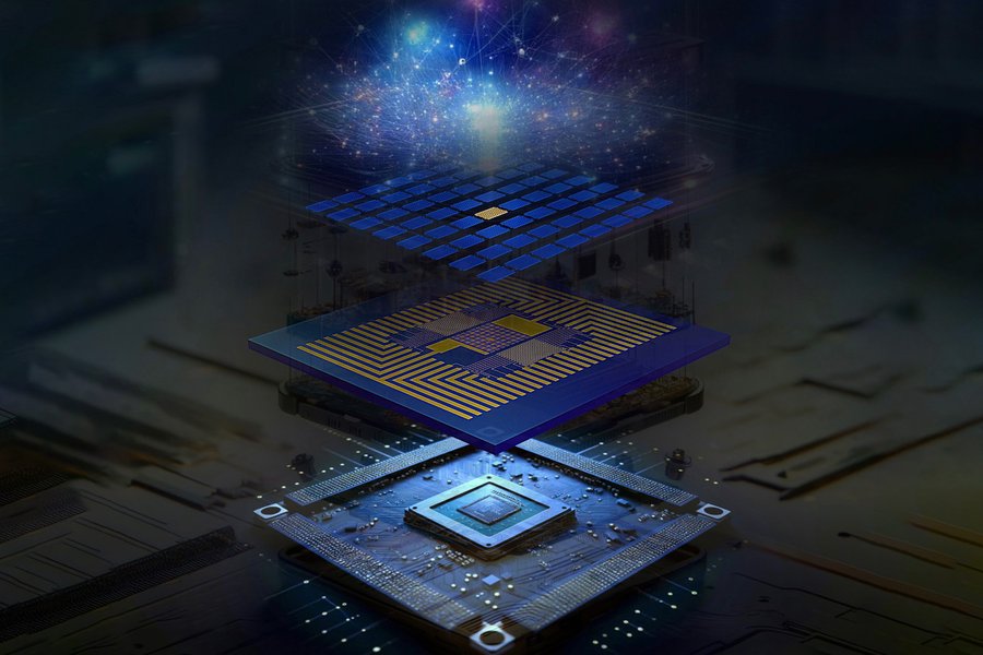
Modern quantum processors house qubits and the intricate wiring needed for control and readout.
Illustrative Example: Deutsch's Algorithm
Deutsch's algorithm, developed by David Deutsch in 1985, was one of the first examples demonstrating that a quantum computer could solve a problem faster than any possible classical computer. While simple, it beautifully illustrates the power of superposition and interference.
The Problem
Consider a function \(f: \{0, 1\} \to \{0, 1\}\), which takes a single bit as input and produces a single bit as output. There are four such functions. Two are constant (output is always 0, or always 1, regardless of input), and two are balanced (output is 0 for one input and 1 for the other). The problem is to determine whether the function \(f\) is constant or balanced by evaluating it.
Classical Approach
Classically, you must evaluate the function twice: once for input 0 (to get \(f(0)\)) and once for input 1 (to get \(f(1)\)). Only by comparing \(f(0)\) and \(f(1)\) can you definitively determine if the function is constant or balanced.
Quantum Approach (Deutsch's Algorithm)
Deutsch's algorithm solves this problem with only one evaluation of the function, implemented as a quantum "oracle" or gate, \(U_f\).
Steps:
- Initialization: Start with two qubits, initialized to \(|0\rangle\) and \(|1\rangle\). The state is \(|01\rangle\).
- Apply Hadamard Gates: Apply a Hadamard gate (H) to both qubits.
- H on \(|0\rangle\) gives \(\frac{|0\rangle + |1\rangle}{\sqrt{2}}\).
- H on \(|1\rangle\) gives \(\frac{|0\rangle - |1\rangle}{\sqrt{2}}\).
- Apply the Oracle \(U_f\): The oracle \(U_f\) acts on two qubits \(|x\rangle|y\rangle\) and transforms them to \(|x\rangle|y \oplus f(x)\rangle\), where \(\oplus\) denotes addition modulo 2. Applying \(U_f\) to the current state cleverly encodes information about \(f(0)\) and \(f(1)\) into the phase of the first qubit.
- If \(f\) is constant (\(f(0)=f(1)\)), the state after the oracle becomes \(\pm \frac{1}{2}(|0\rangle + |1\rangle)(|0\rangle - |1\rangle)\).
- If \(f\) is balanced (\(f(0) \neq f(1)\)), the state becomes \(\pm \frac{1}{2}(|0\rangle - |1\rangle)(|0\rangle - |1\rangle)\).
- Apply Hadamard Gate to First Qubit: Apply another Hadamard gate only to the first qubit. This step causes interference.
- If \(f\) was constant, the first qubit becomes \(|0\rangle\).
- If \(f\) was balanced, the first qubit becomes \(|1\rangle\).
- Measure First Qubit: Measure the first qubit.
- If the measurement result is 0, the function \(f\) is constant.
- If the measurement result is 1, the function \(f\) is balanced.
By using superposition to evaluate the function for both inputs simultaneously and interference to combine the results, Deutsch's algorithm determines the global property of the function (constant or balanced) with a single query, showcasing a clear quantum advantage for this specific task.
Understanding Quantum Computing Visually
For a dynamic introduction to quantum computing concepts, including qubits, superposition, and entanglement, consider this introductory video:
This video provides a foundational overview suitable for beginners, explaining the core ideas behind quantum computation and its potential impact, complementing the technical details discussed here.
Bits vs. Qubits: A Quick Comparison
The following table summarizes the key differences between the fundamental units of classical and quantum information.
| Feature | Classical Bit | Quantum Bit (Qubit) |
|---|---|---|
| Basic State | Deterministic: Either 0 or 1 | Quantum state: Can be \(|0\rangle\), \(|1\rangle\), or a superposition \(\alpha|0\rangle + \beta|1\rangle\) |
| Representation | Single binary value | Vector in a 2D complex Hilbert space |
| Phenomena Used | Classical physics (voltage levels) | Quantum mechanics (superposition, entanglement) |
| Multiple Units | \(n\) bits represent one of \(2^n\) states | \(n\) qubits can represent \(2^n\) states simultaneously in superposition |
| Copying | Easily copied | Cannot be perfectly copied (No-Cloning Theorem) |
| Measurement | Reads the definite state (0 or 1) | Collapses superposition to \(|0\rangle\) or \(|1\rangle\) probabilistically |
This comparison highlights the unique properties of qubits that enable the potential power of quantum computing.
Frequently Asked Questions (FAQ)
What is the main advantage of quantum computers?
The primary advantage lies in their potential to solve certain types of computational problems much faster than classical computers. This includes problems involving factorization (important for cryptography), searching large unstructured datasets, simulating quantum mechanical systems (useful in chemistry and materials science), and solving complex optimization problems. The speedup often comes from exploiting superposition and entanglement to perform calculations in parallel.
Are quantum computers faster than classical computers for all tasks?
No. Quantum computers are not expected to replace classical computers for everyday tasks like web browsing, word processing, or even many scientific computations where classical algorithms are already efficient. Quantum algorithms provide speedups only for specific classes of problems where quantum phenomena can be effectively leveraged. For many problems, classical computers remain the best tool.
What are the biggest challenges in building quantum computers?
Major challenges include:
- Decoherence: Qubits are extremely sensitive to environmental noise, which causes them to lose their quantum properties quickly. Maintaining coherence long enough for computation is difficult.
- Scalability: Building systems with a large number of high-quality, well-connected qubits is technologically demanding.
- Error Correction: Implementing effective quantum error correction requires substantial overhead in terms of the number of physical qubits needed to create one logical (error-corrected) qubit.
- Control and Measurement: Precisely controlling and measuring individual qubits without disturbing others is complex.
When can we expect powerful, fault-tolerant quantum computers?
It's difficult to predict precisely. While significant progress is being made, building large-scale, fault-tolerant quantum computers capable of breaking current encryption standards or revolutionizing drug discovery is likely still years, possibly decades, away. However, NISQ devices are already being used for research and exploring potential near-term applications, and advancements in hardware and algorithms are continuous.
Recommended Further Exploration
- How does Grover's algorithm achieve quadratic speedup in database searches?
- What makes Shor's algorithm a threat to current encryption methods?
- What are the leading physical implementations of qubits today?
- How do quantum error correction codes protect fragile quantum information?
References
 aws.amazon.com

Last updated April 30, 2025