
Unlocking Solar Efficiency: How Mathematical Models Illuminate CSP Receiver Performance
Delving into the equations and simulations that drive the design and optimization of Concentrating Solar Power receivers.
Mathematical models are indispensable tools in the design, analysis, and optimization of Concentrating Solar Power (CSP) receivers. These receivers are the heart of CSP plants, where concentrated sunlight is converted into high-temperature thermal energy. By simulating complex physical processes, engineers and researchers can predict performance, enhance efficiency, and ensure the durability of these critical components. This exploration covers the diverse mathematical frameworks used to understand and improve CSP receiver technology as of May 18, 2025.
Key Insights into CSP Receiver Modeling
- Comprehensive Simulation: Mathematical models intricately simulate the coupled phenomena of heat transfer (conduction, convection, radiation), fluid dynamics of the heat transfer fluid (HTF), and optical interactions occurring within CSP receivers.
- Design and Optimization Focus: These models are pivotal for optimizing receiver geometries, material selection, and operating strategies to maximize thermal efficiency, predict performance under varying solar and atmospheric conditions, and minimize thermal stresses and energy losses.
- Diverse Methodologies: A spectrum of modeling techniques is employed, ranging from simplified steady-state thermal resistance networks for rapid assessment, to complex Computational Fluid Dynamics (CFD) for detailed flow and temperature field analysis, and dynamic models for transient behavior and system integration.
The Indispensable Role of Mathematical Modeling in CSP Receivers
CSP technology relies on concentrating solar radiation onto a receiver, where a heat transfer fluid (HTF) like molten salt, thermal oil, or gas is heated to high temperatures. The performance of this receiver is paramount to the overall plant efficiency. Mathematical models provide the means to understand and predict this performance.
Why Model CSP Receivers?
The primary objectives of modeling CSP receivers include:
- Performance Prediction: Estimating thermal efficiency, outlet HTF temperature, and energy output under various solar irradiance levels, ambient temperatures, and HTF flow rates.
- Design Optimization: Iteratively refining receiver geometry (e.g., tube dimensions, cavity shape), material selection, and surface coatings to maximize solar absorption and minimize heat losses.
- Operational Strategy Development: Simulating different control strategies for start-up, shutdown, and transient conditions (e.g., cloud passage) to ensure safe and efficient operation.
- Thermal Stress Analysis: Calculating temperature gradients and resultant thermal stresses within receiver components to prevent material failure and ensure long-term reliability.
- Cost Reduction: Enabling virtual prototyping and optimization, thereby reducing the need for extensive and costly physical experimentation.
Key Parameters Under Investigation
Mathematical models for CSP receivers aim to determine a range of critical parameters, such as:
- Heat transfer fluid mass flow rate required to achieve a target outlet temperature.
- Temperature distribution on the receiver surfaces and within its structural components (e.g., tubes).
- Overall receiver thermal efficiency.
- Pressure drop of the HTF across the receiver.
- Heat losses due to convection, radiation, and conduction to the surroundings.
- Optical efficiency of the receiver in absorbing concentrated sunlight.
- Mechanical stresses and strains in receiver panels due to thermal expansion.
Core Components of CSP Receiver Models
Modeling a CSP receiver involves dissecting its operation into fundamental physical processes, each described by specific mathematical formulations.
Mastering Heat Transfer Dynamics
Heat transfer is the cornerstone of receiver modeling, encompassing how solar energy is absorbed, transferred to the HTF, and lost to the environment.
The Fundamental Energy Balance
At a high level, the energy balance for a receiver in steady-state can be expressed as:
\[ Q_{\text{absorbed}} = Q_{\text{useful}} + Q_{\text{losses}} \]Where:
- \( Q_{\text{absorbed}} \) is the solar radiation absorbed by the receiver.
- \( Q_{\text{useful}} \) is the thermal energy transferred to the heat transfer fluid.
- \( Q_{\text{losses}} \) represents the total heat losses (radiative, convective, conductive) from the receiver to the surroundings.
The amount of heat transferred to the fluid can also be generally described by:
\[ Q_{\text{useful}} = \dot{m} C_p \Delta T \]Where \( \dot{m} \) is the mass flow rate of the HTF, \( C_p \) is its specific heat capacity, and \( \Delta T \) is the temperature difference of the HTF between the inlet and outlet.
Conduction and Convection within Receiver Materials and to the Fluid
Heat conduction through the receiver's solid materials (e.g., metal tubes) and convection to the HTF are critical. For a tubular receiver, the steady-state heat transfer through the tube wall and into the fluid can be modeled. For instance, a simplified one-dimensional heat conduction-convection equation for a segment of a receiver tube might be:
\[ \frac{d}{dx} \left( k A \frac{dT_w}{dx} \right) - h_i P_i (T_w - T_f) + q''_{\text{solar}} P_o - h_o P_o (T_w - T_{\text{amb}}) - \epsilon \sigma P_o (T_w^4 - T_{\text{surr}}^4) = 0 \]This equation is a more comprehensive form, where \(k\) is thermal conductivity, \(A\) is cross-sectional area, \(T_w\) is wall temperature, \(T_f\) is fluid temperature, \(h_i\) and \(h_o\) are internal and external convective heat transfer coefficients, \(P_i\) and \(P_o\) are internal and external perimeters, \(q''_{\text{solar}}\) is absorbed solar flux, \(T_{\text{amb}}\) is ambient temperature, \(\epsilon\) is emissivity, \(\sigma\) is the Stefan-Boltzmann constant, and \(T_{\text{surr}}\) is the surrounding temperature for radiation.
Radiative Heat Exchange
Radiative heat transfer is dominant, both for solar energy absorption and for heat losses at high operating temperatures. Models account for the receiver surface's absorptivity (for incoming solar radiation) and emissivity (for outgoing thermal radiation). The net radiative heat flux is a key component of \(Q_{\text{absorbed}}\) and \(Q_{\text{losses}}\).
Simulating Fluid Flow (Thermofluid Models)
The flow of the HTF within the receiver tubes or channels is modeled using principles of fluid mechanics and thermodynamics.
Governing Equations
Thermofluid models solve conservation equations for mass, momentum, and energy for the HTF. These can range from simple one-dimensional flow assumptions to complex three-dimensional CFD simulations.
Heat Transfer to the Fluid
The energy absorbed by the HTF as it flows through the receiver, leading to its temperature rise, is modeled by equations such as:
\[ \dot{m} c_p \frac{dT_f}{dx} = h_i P_i (T_s - T_f) \]Where \(T_s\) is the internal surface temperature of the receiver tube in contact with the fluid. This equation is often solved coupled with the heat conduction equations for the receiver material.
Capturing Solar Energy: Optical Modeling
Accurate prediction of how concentrated sunlight interacts with the receiver surface is crucial.
Solar Flux Mapping
Optical models, often using Monte Carlo Ray Tracing (MCRT) techniques, simulate the path of solar rays from the heliostat field or concentrator array to the receiver. This results in a detailed solar flux map, indicating the distribution and intensity of radiation incident on various parts of the receiver surface. This flux map serves as a critical input to the thermal models.
Predominant Modeling Approaches
Various mathematical modeling strategies are employed, each with its own balance of accuracy, computational cost, and complexity.
Thermal Resistance Network Models: A Balanced Approach
These steady-state models simplify the complex heat transfer pathways within the receiver into an equivalent network of thermal resistances. Each component (e.g., tube wall conduction, convection to HTF, radiation loss) is represented by a resistance.
The total thermal resistance \(R_{\text{total}}\) can be a combination of resistances in series and parallel, for example:
\[ R_{\text{total}} = R_{\text{conduction,wall}} + R_{\text{convection,internal}} + R_{\text{convection,external}} + R_{\text{radiation,external}} \]These models are computationally efficient and widely used for initial design, parametric studies, and performance estimation of central receivers and other types. They can predict key parameters like fluid outlet temperature, surface temperatures, and overall efficiency with reasonable accuracy. Below is an image of a next-generation particle receiver tower, a type of system where advanced thermal modeling is critical.
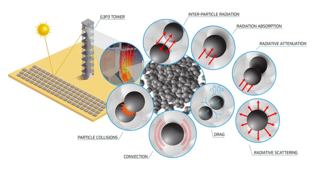
Next-Generation Particle Receiver Tower at Sandia National Laboratories.
Dynamic Modeling: Capturing Real-World Variability
CSP plants operate under fluctuating solar irradiance and varying demand. Dynamic models, often based on solving systems of time-dependent ordinary differential equations (ODEs) or partial differential equations (PDEs), simulate the transient behavior of the receiver. This is crucial for analyzing start-up/shutdown procedures, response to cloud cover, and integration with thermal energy storage (TES) systems.
Computational Fluid Dynamics (CFD): In-Depth Analysis
CFD models provide highly detailed, three-dimensional simulations of fluid flow and heat transfer within the receiver. They solve the Navier-Stokes equations coupled with energy equations. While computationally intensive, CFD is invaluable for understanding complex flow patterns, non-uniform temperature distributions, and localized hot spots, especially in receivers with intricate geometries or those using particle flows.
Reduced Order Models (ROM): Efficient Optimization
ROM techniques aim to create simplified yet accurate representations of more complex models (like CFD). By reducing the dimensionality of the problem, ROMs significantly decrease computational time, making them suitable for rapid optimization studies, control system design, and real-time performance monitoring.
Advanced and Specialized Receiver Models
As CSP technology evolves, so do the mathematical models designed to capture the nuances of innovative receiver designs.
Innovations in Particle and Volumetric Receivers
Next-generation CSP systems explore concepts like particle receivers and volumetric receivers to achieve higher temperatures and efficiencies.
- Particle Receivers: Solid particles (e.g., ceramic) directly absorb concentrated solar radiation, either flowing freely or in an enclosed cavity. Models for these systems must account for granular flow dynamics, particle-radiation interaction, and particle-to-fluid or particle-to-wall heat exchange. Continuum models or discrete element methods (DEM) might be employed.
- Volumetric Receivers: Solar radiation is absorbed throughout the volume of a porous structure (e.g., ceramic foam). Modeling involves complex radiative transfer within the porous medium and convective heat transfer to the HTF flowing through it.
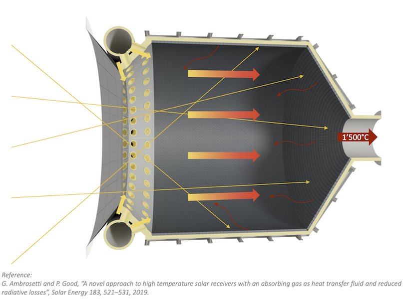
Synhelion's solar receiver designed for achieving ultra-high temperatures, crucial for producing solar fuels.
Integrating Receivers with Thermal Energy Storage (TES)
For continuous power generation, CSP plants often incorporate TES. Some novel designs aim to integrate the receiver and storage functions into a single unit. Models for such systems must couple the receiver's thermal performance with the charging/discharging dynamics of the storage medium. This involves solving transient heat transfer and fluid flow equations for both components simultaneously.
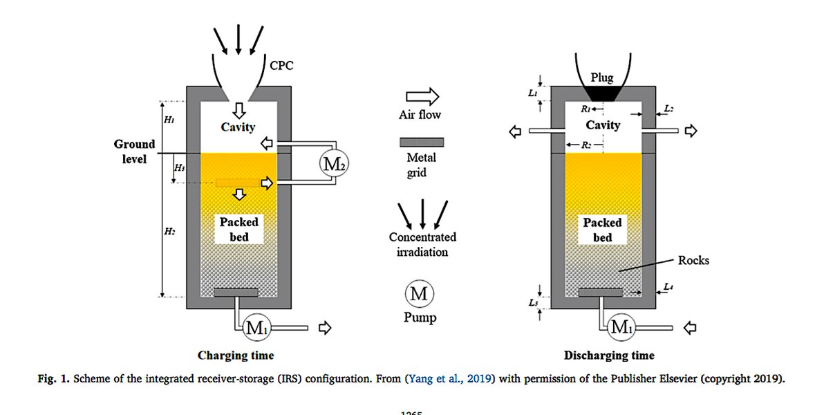
Concept of an integrated solar receiver and thermal energy storage unit for improved efficiency.
Mathematical Programming for Optimal Design
Optimization techniques, such as mixed-integer nonlinear programming (MINLP) or nonlinear programming (NLP), are used in conjunction with receiver models. These mathematical programming approaches help identify optimal design parameters (e.g., tube diameter, receiver height, HTF flow strategy) that maximize efficiency or minimize cost, subject to material and operational constraints. They can also consider location-specific factors like solar radiation profiles.
Comparing Modeling Approaches: A Visual Overview
Different mathematical modeling approaches for CSP receivers offer trade-offs in terms of computational cost, accuracy, complexity, and the scope of phenomena they can capture. The radar chart below provides a qualitative comparison of some common methodologies. These are generalized assessments and can vary based on specific implementation and application.
This chart illustrates that while CFD models offer high accuracy and detail, they come with significant computational costs and complexity. Thermal resistance networks, on the other hand, are computationally efficient but may sacrifice some accuracy for simpler representations. Dynamic models are essential for capturing transient effects, and ROMs try to bridge the gap by offering reduced complexity with good accuracy.
Visualizing the Modeling Landscape: A Mindmap
The interconnected nature of CSP receiver modeling, encompassing various physical phenomena, methodologies, inputs, and outputs, can be visualized using a mindmap. This helps in understanding the holistic approach required for comprehensive receiver analysis.
This mindmap highlights how various facets of physics and engineering mathematics converge to create a comprehensive understanding of CSP receiver behavior, guiding engineers towards more efficient and reliable solar energy conversion systems.
Summary of Modeling Aspects in CSP Receivers
The following table summarizes the key aspects involved in the mathematical modeling of CSP receivers, outlining the concepts and their purpose in the overall analysis and design process.
| Modeling Aspect | Key Equations / Concepts | Purpose |
|---|---|---|
| Overall Energy Balance | \( Q_{\text{absorbed}} = Q_{\text{useful}} + Q_{\text{losses}} \) | Fundamental accounting of energy flows to determine efficiency. |
| Heat Transfer (Conduction) | Fourier's Law: \( q = -kA \frac{dT}{dx} \) | Model heat flow through solid receiver components. |
| Heat Transfer (Convection) | Newton's Law of Cooling: \( q = hA(T_s - T_f) \) | Model heat exchange between receiver surfaces and fluids (HTF, air). |
| Heat Transfer (Radiation) | Stefan-Boltzmann Law: \( q = \epsilon \sigma A (T_s^4 - T_{\text{surr}}^4) \); View factors. | Model solar energy absorption and radiative heat losses. |
| Fluid Dynamics (HTF Flow) | Conservation of mass, momentum, and energy (Navier-Stokes equations for CFD). Energy equation for HTF: \( \dot{m} c_p dT_f = dQ_{\text{useful}} \) | Calculate HTF temperature rise, pressure drop, and flow distribution. |
| Optical Modeling | Ray tracing algorithms (e.g., Monte Carlo), surface optical properties (absorptivity, reflectivity). | Determine solar flux distribution on receiver surfaces. |
| Thermal Resistance Networks | Equivalent electrical circuit analogy for heat transfer paths. | Simplify complex heat transfer for faster design iterations and system-level analysis. |
| Dynamic Modeling | Time-dependent differential equations (ODEs/PDEs) for energy storage and temperature changes. | Simulate transient behavior, start-up/shutdown, and response to varying conditions. |
| Thermomechanical Analysis | Coupling thermal models with structural mechanics (stress-strain relationships, thermal expansion). | Assess thermal stresses and strains to ensure structural integrity. |
| Advanced Configurations | Models for porous media, particle flow, thermochemical reactions. | Analyze novel receiver technologies for enhanced performance and storage integration. |
Practical Application: Modeling Tools and Techniques
Various software tools and numerical techniques are employed to implement these mathematical models. Tools like the System Advisor Model (SAM) developed by NREL, SolarPILOT, COMSOL Multiphysics, ANSYS Fluent, and programming environments like MATLAB and Python with specialized libraries are commonly used in academia and industry. The video below provides an overview of modeling power tower systems using SAM, illustrating how these complex mathematical concepts are put into practice.
Overview of modeling concentrating solar power tower systems using the System Advisor Model (SAM) and SolarPILOT.
These tools often incorporate solvers for differential equations, heat transfer correlations, fluid dynamics computations, and ray-tracing capabilities, allowing engineers to simulate CSP receiver performance comprehensively.
Frequently Asked Questions (FAQ)
What is the primary goal of modeling CSP receivers?
The primary goals are to predict the thermal performance (e.g., efficiency, outlet temperature), optimize the design for maximum energy conversion and minimal losses, ensure structural integrity under thermal loads, and evaluate operational strategies under various conditions.
What are common types of heat transfer fluids (HTFs) considered in these models?
Common HTFs include molten salts (e.g., solar salt - a mixture of sodium nitrate and potassium nitrate), synthetic thermal oils, water/steam, air, and supercritical carbon dioxide (sCO2). Emerging concepts also use solid particles as direct absorption HTFs.
How do optical models contribute to receiver design?
Optical models, often using ray-tracing techniques, determine the distribution of concentrated solar flux on the receiver surface. This flux map is a critical input for thermal models, helping to identify potential hot spots, optimize receiver aiming strategies, and accurately calculate absorbed solar energy.
Why are dynamic models important for CSP receivers?
Dynamic models are crucial for simulating the receiver's behavior under time-varying conditions, such as changes in solar irradiance (e.g., due to clouds), start-up and shutdown procedures, and interactions with thermal energy storage systems. This helps in designing robust control systems and assessing performance over realistic operational cycles.
What are thermal resistance network models?
Thermal resistance network models are a simplified approach where different heat transfer paths (conduction, convection, radiation) within the receiver are represented as an analogous electrical circuit with thermal resistances. They offer a computationally efficient way to estimate steady-state performance, like overall efficiency and temperature distributions, making them useful for initial design and parametric studies.
Recommended Further Exploration
To delve deeper into the intricacies of CSP receiver modeling, consider exploring these related queries:
- How do Computational Fluid Dynamics (CFD) models compare to thermal resistance network models for analyzing solar tower receivers?
- What are the specific challenges and mathematical approaches for modeling next-generation particle receivers in high-temperature CSP applications?
- How are dynamic models used to simulate the interaction between CSP receivers and thermal energy storage systems during charging and discharging cycles?
- What optimization algorithms and mathematical programming techniques are employed to enhance the design and operational efficiency of concentrating solar power receivers?
References
- Thermal resistance model for CSP central receivers - ResearchGate
- Predictive performance modeling framework for a novel enclosed particle receiver configuration - ResearchGate
- Simplified heat loss model for central tower solar receiver - ScienceDirect
- Optimal Design of Solar Receivers in CSP Plants - ACS Publications
- Novel CSP Design Combines the Solar Receiver with Thermal Energy Storage - SolarPACES
- Receiver R&D for CSP Systems - U.S. Department of Energy
- Comprehensive mathematical model and efficient numerical analysis of the design parameters of the parabolic trough receiver - ResearchGate
Unlocking Solar Efficiency: How Mathematical Models Illuminate CSP Receiver Performance
Delving into the equations and simulations that drive the design and optimization of Concentrating Solar Power receivers.
Mathematical models are indispensable tools in the design, analysis, and optimization of Concentrating Solar Power (CSP) receivers. These receivers are the heart of CSP plants, where concentrated sunlight is converted into high-temperature thermal energy. By simulating complex physical processes, engineers and researchers can predict performance, enhance efficiency, and ensure the durability of these critical components. This exploration covers the diverse mathematical frameworks used to understand and improve CSP receiver technology as of May 18, 2025.
Key Insights into CSP Receiver Modeling
- Comprehensive Simulation: Mathematical models intricately simulate the coupled phenomena of heat transfer (conduction, convection, radiation), fluid dynamics of the heat transfer fluid (HTF), and optical interactions occurring within CSP receivers.
- Design and Optimization Focus: These models are pivotal for optimizing receiver geometries, material selection, and operating strategies to maximize thermal efficiency, predict performance under varying solar and atmospheric conditions, and minimize thermal stresses and energy losses.
- Diverse Methodologies: A spectrum of modeling techniques is employed, ranging from simplified steady-state thermal resistance networks for rapid assessment, to complex Computational Fluid Dynamics (CFD) for detailed flow and temperature field analysis, and dynamic models for transient behavior and system integration.
The Indispensable Role of Mathematical Modeling in CSP Receivers
CSP technology relies on concentrating solar radiation onto a receiver, where a heat transfer fluid (HTF) like molten salt, thermal oil, or gas is heated to high temperatures. The performance of this receiver is paramount to the overall plant efficiency. Mathematical models provide the means to understand and predict this performance.
Why Model CSP Receivers?
The primary objectives of modeling CSP receivers include:
- Performance Prediction: Estimating thermal efficiency, outlet HTF temperature, and energy output under various solar irradiance levels, ambient temperatures, and HTF flow rates.
- Design Optimization: Iteratively refining receiver geometry (e.g., tube dimensions, cavity shape), material selection, and surface coatings to maximize solar absorption and minimize heat losses.
- Operational Strategy Development: Simulating different control strategies for start-up, shutdown, and transient conditions (e.g., cloud passage) to ensure safe and efficient operation.
- Thermal Stress Analysis: Calculating temperature gradients and resultant thermal stresses within receiver components to prevent material failure and ensure long-term reliability.
- Cost Reduction: Enabling virtual prototyping and optimization, thereby reducing the need for extensive and costly physical experimentation.
Key Parameters Under Investigation
Mathematical models for CSP receivers aim to determine a range of critical parameters, such as:
- Heat transfer fluid mass flow rate required to achieve a target outlet temperature.
- Temperature distribution on the receiver surfaces and within its structural components (e.g., tubes).
- Overall receiver thermal efficiency.
- Pressure drop of the HTF across the receiver.
- Heat losses due to convection, radiation, and conduction to the surroundings.
- Optical efficiency of the receiver in absorbing concentrated sunlight.
- Mechanical stresses and strains in receiver panels due to thermal expansion.
Core Components of CSP Receiver Models
Modeling a CSP receiver involves dissecting its operation into fundamental physical processes, each described by specific mathematical formulations.
Mastering Heat Transfer Dynamics
Heat transfer is the cornerstone of receiver modeling, encompassing how solar energy is absorbed, transferred to the HTF, and lost to the environment.
The Fundamental Energy Balance
At a high level, the energy balance for a receiver in steady-state can be expressed as:
\[ Q_{\text{absorbed}} = Q_{\text{useful}} + Q_{\text{losses}} \]Where:
- \( Q_{\text{absorbed}} \) is the solar radiation absorbed by the receiver.
- \( Q_{\text{useful}} \) is the thermal energy transferred to the heat transfer fluid.
- \( Q_{\text{losses}} \) represents the total heat losses (radiative, convective, conductive) from the receiver to the surroundings.
The amount of heat transferred to the fluid can also be generally described by:
\[ Q_{\text{useful}} = \dot{m} C_p \Delta T \]Where \( \dot{m} \) is the mass flow rate of the HTF, \( C_p \) is its specific heat capacity, and \( \Delta T \) is the temperature difference of the HTF between the inlet and outlet.
Conduction and Convection within Receiver Materials and to the Fluid
Heat conduction through the receiver's solid materials (e.g., metal tubes) and convection to the HTF are critical. For a tubular receiver, the steady-state heat transfer through the tube wall and into the fluid can be modeled. For instance, a simplified one-dimensional heat conduction-convection equation for a segment of a receiver tube might be:
\[ \frac{d}{dx} \left( k A \frac{dT_w}{dx} \right) - h_i P_i (T_w - T_f) + q''_{\text{solar}} P_o - h_o P_o (T_w - T_{\text{amb}}) - \epsilon \sigma P_o (T_w^4 - T_{\text{surr}}^4) = 0 \]This equation is a more comprehensive form, where \(k\) is thermal conductivity, \(A\) is cross-sectional area, \(T_w\) is wall temperature, \(T_f\) is fluid temperature, \(h_i\) and \(h_o\) are internal and external convective heat transfer coefficients, \(P_i\) and \(P_o\) are internal and external perimeters, \(q''_{\text{solar}}\) is absorbed solar flux, \(T_{\text{amb}}\) is ambient temperature, \(\epsilon\) is emissivity, \(\sigma\) is the Stefan-Boltzmann constant, and \(T_{\text{surr}}\) is the surrounding temperature for radiation.
Radiative Heat Exchange
Radiative heat transfer is dominant, both for solar energy absorption and for heat losses at high operating temperatures. Models account for the receiver surface's absorptivity (for incoming solar radiation) and emissivity (for outgoing thermal radiation). The net radiative heat flux is a key component of \(Q_{\text{absorbed}}\) and \(Q_{\text{losses}}\).
Simulating Fluid Flow (Thermofluid Models)
The flow of the HTF within the receiver tubes or channels is modeled using principles of fluid mechanics and thermodynamics.
Governing Equations
Thermofluid models solve conservation equations for mass, momentum, and energy for the HTF. These can range from simple one-dimensional flow assumptions to complex three-dimensional CFD simulations.
Heat Transfer to the Fluid
The energy absorbed by the HTF as it flows through the receiver, leading to its temperature rise, is modeled by equations such as:
\[ \dot{m} c_p \frac{dT_f}{dx} = h_i P_i (T_s - T_f) \]Where \(T_s\) is the internal surface temperature of the receiver tube in contact with the fluid. This equation is often solved coupled with the heat conduction equations for the receiver material.
Capturing Solar Energy: Optical Modeling
Accurate prediction of how concentrated sunlight interacts with the receiver surface is crucial.
Solar Flux Mapping
Optical models, often using Monte Carlo Ray Tracing (MCRT) techniques, simulate the path of solar rays from the heliostat field or concentrator array to the receiver. This results in a detailed solar flux map, indicating the distribution and intensity of radiation incident on various parts of the receiver surface. This flux map serves as a critical input to the thermal models.
Predominant Modeling Approaches
Various mathematical modeling strategies are employed, each with its own balance of accuracy, computational cost, and complexity.
Thermal Resistance Network Models: A Balanced Approach
These steady-state models simplify the complex heat transfer pathways within the receiver into an equivalent network of thermal resistances. Each component (e.g., tube wall conduction, convection to HTF, radiation loss) is represented by a resistance.
The total thermal resistance \(R_{\text{total}}\) can be a combination of resistances in series and parallel, for example:
\[ R_{\text{total}} = R_{\text{conduction,wall}} + R_{\text{convection,internal}} + R_{\text{convection,external}} + R_{\text{radiation,external}} \]These models are computationally efficient and widely used for initial design, parametric studies, and performance estimation of central receivers and other types. They can predict key parameters like fluid outlet temperature, surface temperatures, and overall efficiency with reasonable accuracy. Below is an image of a next-generation particle receiver tower, a type of system where advanced thermal modeling is critical.
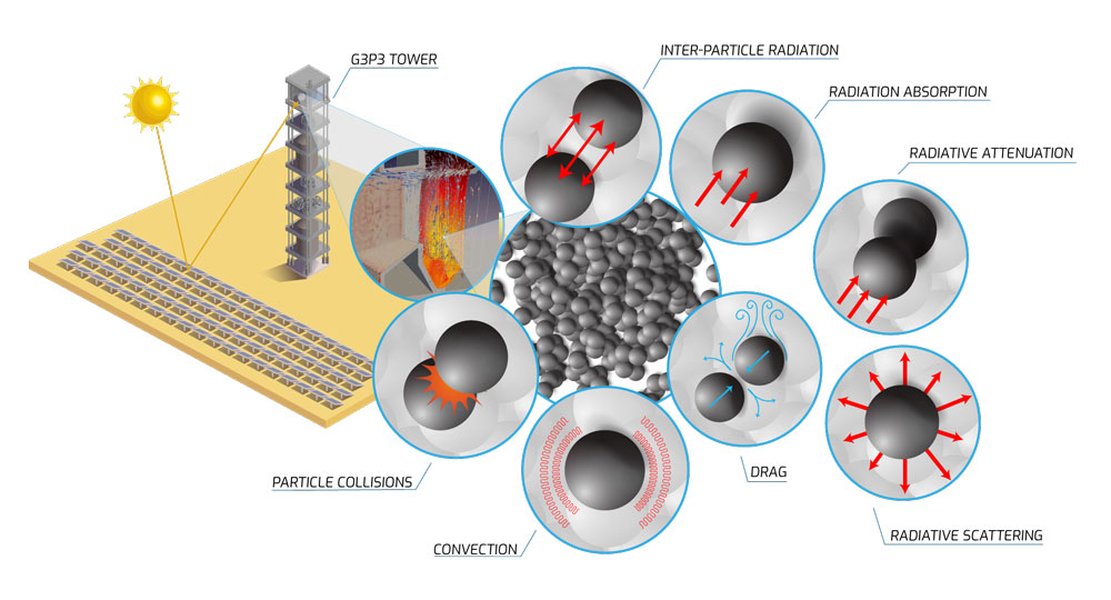
Next-Generation Particle Receiver Tower at Sandia National Laboratories.
Dynamic Modeling: Capturing Real-World Variability
CSP plants operate under fluctuating solar irradiance and varying demand. Dynamic models, often based on solving systems of time-dependent ordinary differential equations (ODEs) or partial differential equations (PDEs), simulate the transient behavior of the receiver. This is crucial for analyzing start-up/shutdown procedures, response to cloud cover, and integration with thermal energy storage (TES) systems.
Computational Fluid Dynamics (CFD): In-Depth Analysis
CFD models provide highly detailed, three-dimensional simulations of fluid flow and heat transfer within the receiver. They solve the Navier-Stokes equations coupled with energy equations. While computationally intensive, CFD is invaluable for understanding complex flow patterns, non-uniform temperature distributions, and localized hot spots, especially in receivers with intricate geometries or those using particle flows.
Reduced Order Models (ROM): Efficient Optimization
ROM techniques aim to create simplified yet accurate representations of more complex models (like CFD). By reducing the dimensionality of the problem, ROMs significantly decrease computational time, making them suitable for rapid optimization studies, control system design, and real-time performance monitoring.
Advanced and Specialized Receiver Models
As CSP technology evolves, so do the mathematical models designed to capture the nuances of innovative receiver designs.
Innovations in Particle and Volumetric Receivers
Next-generation CSP systems explore concepts like particle receivers and volumetric receivers to achieve higher temperatures and efficiencies.
- Particle Receivers: Solid particles (e.g., ceramic) directly absorb concentrated solar radiation, either flowing freely or in an enclosed cavity. Models for these systems must account for granular flow dynamics, particle-radiation interaction, and particle-to-fluid or particle-to-wall heat exchange. Continuum models or discrete element methods (DEM) might be employed.
- Volumetric Receivers: Solar radiation is absorbed throughout the volume of a porous structure (e.g., ceramic foam). Modeling involves complex radiative transfer within the porous medium and convective heat transfer to the HTF flowing through it.
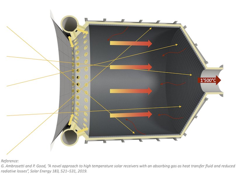
Synhelion's solar receiver designed for achieving ultra-high temperatures, crucial for producing solar fuels.
Integrating Receivers with Thermal Energy Storage (TES)
For continuous power generation, CSP plants often incorporate TES. Some novel designs aim to integrate the receiver and storage functions into a single unit. Models for such systems must couple the receiver's thermal performance with the charging/discharging dynamics of the storage medium. This involves solving transient heat transfer and fluid flow equations for both components simultaneously.
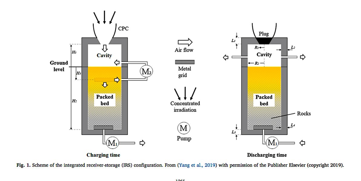
Concept of an integrated solar receiver and thermal energy storage unit for improved efficiency.
Mathematical Programming for Optimal Design
Optimization techniques, such as mixed-integer nonlinear programming (MINLP) or nonlinear programming (NLP), are used in conjunction with receiver models. These mathematical programming approaches help identify optimal design parameters (e.g., tube diameter, receiver height, HTF flow strategy) that maximize efficiency or minimize cost, subject to material and operational constraints. They can also consider location-specific factors like solar radiation profiles.
Comparing Modeling Approaches: A Visual Overview
Different mathematical modeling approaches for CSP receivers offer trade-offs in terms of computational cost, accuracy, complexity, and the scope of phenomena they can capture. The radar chart below provides a qualitative comparison of some common methodologies. These are generalized assessments and can vary based on specific implementation and application.
This chart illustrates that while CFD models offer high accuracy and detail, they come with significant computational costs and complexity. Thermal resistance networks, on the other hand, are computationally efficient but may sacrifice some accuracy for simpler representations. Dynamic models are essential for capturing transient effects, and ROMs try to bridge the gap by offering reduced complexity with good accuracy.
Visualizing the Modeling Landscape: A Mindmap
The interconnected nature of CSP receiver modeling, encompassing various physical phenomena, methodologies, inputs, and outputs, can be visualized using a mindmap. This helps in understanding the holistic approach required for comprehensive receiver analysis.
This mindmap highlights how various facets of physics and engineering mathematics converge to create a comprehensive understanding of CSP receiver behavior, guiding engineers towards more efficient and reliable solar energy conversion systems.
Summary of Modeling Aspects in CSP Receivers
The following table summarizes the key aspects involved in the mathematical modeling of CSP receivers, outlining the concepts and their purpose in the overall analysis and design process.
| Modeling Aspect | Key Equations / Concepts | Purpose |
|---|---|---|
| Overall Energy Balance | \( Q_{\text{absorbed}} = Q_{\text{useful}} + Q_{\text{losses}} \) | Fundamental accounting of energy flows to determine efficiency. |
| Heat Transfer (Conduction) | Fourier's Law: \( q = -kA \frac{dT}{dx} \) | Model heat flow through solid receiver components. |
| Heat Transfer (Convection) | Newton's Law of Cooling: \( q = hA(T_s - T_f) \) | Model heat exchange between receiver surfaces and fluids (HTF, air). |
| Heat Transfer (Radiation) | Stefan-Boltzmann Law: \( q = \epsilon \sigma A (T_s^4 - T_{\text{surr}}^4) \); View factors. | Model solar energy absorption and radiative heat losses. |
| Fluid Dynamics (HTF Flow) | Conservation of mass, momentum, and energy (Navier-Stokes equations for CFD). Energy equation for HTF: \( \dot{m} c_p dT_f = dQ_{\text{useful}} \) | Calculate HTF temperature rise, pressure drop, and flow distribution. |
| Optical Modeling | Ray tracing algorithms (e.g., Monte Carlo), surface optical properties (absorptivity, reflectivity). | Determine solar flux distribution on receiver surfaces. |
| Thermal Resistance Networks | Equivalent electrical circuit analogy for heat transfer paths. | Simplify complex heat transfer for faster design iterations and system-level analysis. |
| Dynamic Modeling | Time-dependent differential equations (ODEs/PDEs) for energy storage and temperature changes. | Simulate transient behavior, start-up/shutdown, and response to varying conditions. |
| Thermomechanical Analysis | Coupling thermal models with structural mechanics (stress-strain relationships, thermal expansion). | Assess thermal stresses and strains to ensure structural integrity. |
| Advanced Configurations | Models for porous media, particle flow, thermochemical reactions. | Analyze novel receiver technologies for enhanced performance and storage integration. |
Practical Application: Modeling Tools and Techniques
Various software tools and numerical techniques are employed to implement these mathematical models. Tools like the System Advisor Model (SAM) developed by NREL, SolarPILOT, COMSOL Multiphysics, ANSYS Fluent, and programming environments like MATLAB and Python with specialized libraries are commonly used in academia and industry. The video below provides an overview of modeling power tower systems using SAM, illustrating how these complex mathematical concepts are put into practice.
Overview of modeling concentrating solar power tower systems using the System Advisor Model (SAM) and SolarPILOT.
These tools often incorporate solvers for differential equations, heat transfer correlations, fluid dynamics computations, and ray-tracing capabilities, allowing engineers to simulate CSP receiver performance comprehensively.
Frequently Asked Questions (FAQ)
What is the primary goal of modeling CSP receivers?
The primary goals are to predict the thermal performance (e.g., efficiency, outlet temperature), optimize the design for maximum energy conversion and minimal losses, ensure structural integrity under thermal loads, and evaluate operational strategies under various conditions.
What are common types of heat transfer fluids (HTFs) considered in these models?
Common HTFs include molten salts (e.g., solar salt - a mixture of sodium nitrate and potassium nitrate), synthetic thermal oils, water/steam, air, and supercritical carbon dioxide (sCO2). Emerging concepts also use solid particles as direct absorption HTFs.
How do optical models contribute to receiver design?
Optical models, often using ray-tracing techniques, determine the distribution of concentrated solar flux on the receiver surface. This flux map is a critical input for thermal models, helping to identify potential hot spots, optimize receiver aiming strategies, and accurately calculate absorbed solar energy.
Why are dynamic models important for CSP receivers?
Dynamic models are crucial for simulating the receiver's behavior under time-varying conditions, such as changes in solar irradiance (e.g., due to clouds), start-up and shutdown procedures, and interactions with thermal energy storage systems. This helps in designing robust control systems and assessing performance over realistic operational cycles.
What are thermal resistance network models?
Thermal resistance network models are a simplified approach where different heat transfer paths (conduction, convection, radiation) within the receiver are represented as an analogous electrical circuit with thermal resistances. They offer a computationally efficient way to estimate steady-state performance, like overall efficiency and temperature distributions, making them useful for initial design and parametric studies.
Recommended Further Exploration
To delve deeper into the intricacies of CSP receiver modeling, consider exploring these related queries:
- How do Computational Fluid Dynamics (CFD) models compare to thermal resistance network models for analyzing solar tower receivers?
- What are the specific challenges and mathematical approaches for modeling next-generation particle receivers in high-temperature CSP applications?
- How are dynamic models used to simulate the interaction between CSP receivers and thermal energy storage systems during charging and discharging cycles?
- What optimization algorithms and mathematical programming techniques are employed to enhance the design and operational efficiency of concentrating solar power receivers?
References
Last updated May 18, 2025