
Unveiling the Mathematical Secrets Behind High-Temperature Gas Systems in Concentrated Solar Power
A deep dive into the equations and models powering next-generation solar energy, focusing on gas-based systems in CSP receivers.
Highlights: Decoding GHS in CSP
- Interpreting "GHS": In the context of Concentrated Solar Power (CSP) receivers, "GHS" most likely refers to systems involving gas, such as Gas-Phase Solar Receivers (using gases like air or helium as the heat transfer fluid) or integrated Gas Heat Storage. These are pivotal for achieving high operating temperatures and efficiencies.
- Core Modeling Approach: The mathematical backbone for these systems rests on the fundamental principles of energy balance. This involves quantifying incoming solar energy, heat transferred to the gas, thermal storage, and various heat losses through radiation, convection, and conduction.
- Advanced Simulation Power: For detailed performance analysis and design optimization, sophisticated techniques like Computational Fluid Dynamics (CFD) are indispensable. CFD allows for in-depth simulation of fluid flow, heat transfer, and solar radiation interaction within the complex geometries of CSP receivers.
Understanding GHS in the Context of CSP Receivers
Concentrated Solar Power (CSP) technology is a promising avenue for renewable energy generation. To fully grasp the mathematical modeling involved, it's essential to understand its core components and how gas-based systems, potentially referred to by "GHS," fit into this picture.
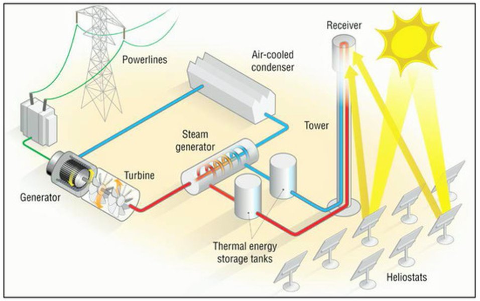
Illustrative diagram of a central receiver CSP system, where heliostats concentrate sunlight onto a tower-mounted receiver.
What is a CSP Receiver?
A CSP receiver is the heart of a concentrated solar power plant. It's the component responsible for absorbing the highly concentrated sunlight, focused by a field of mirrors (heliostats in tower systems, or parabolic troughs/dishes in other designs), and converting this solar radiation into high-temperature thermal energy. This heat is then transferred to a Heat Transfer Fluid (HTF) which can be used to drive a power cycle (typically a steam turbine or a gas turbine) to generate electricity, or it can be stored in a Thermal Energy Storage (TES) system for later use.
Interpreting "GHS": Gas-Phase Systems in CSP
The acronym "GHS" isn't universally standardized in CSP literature. However, in the context of a "GHS on a CSP receiver," it strongly suggests a system involving gas either as the primary heat transfer medium within the receiver or as a storage medium. Two prominent interpretations emerge:
Gas-Phase Solar Receivers
This refers to CSP receivers that use a gas (such as air, helium, or carbon dioxide) as the heat transfer fluid. These systems are particularly interesting because they can achieve very high operating temperatures, often exceeding 700°C and potentially over 1000°C. Such high temperatures can lead to higher thermodynamic cycle efficiencies (e.g., when coupled with Brayton cycles using gas turbines) and enable novel applications like solar thermochemistry for fuel production. Volumetric receivers, where solar radiation is absorbed throughout the volume of a porous material through which the gas flows, are a common type of gas-phase receiver known for their potential for high efficiency.
Gas Heat Storage (GHS)
Alternatively, "GHS" could imply a Gas Heat Storage system. While less common as a standalone term "GHS" compared to established TES (Thermal Energy Storage) terms, gases can be used in sensible heat storage systems, often involving packed beds of ceramic or rock materials. In such a system integrated with a CSP receiver, the hot gas from the receiver would heat the storage material, and this stored heat could later be extracted by passing cooler gas through the material. This is particularly relevant for gas-cooled CSP systems to provide dispatchable power.
For the purpose of discussing mathematical models, we will primarily focus on the aspects relevant to Gas-Phase Solar Receivers, as this directly relates to the operation "on a CSP receiver," while also touching upon principles applicable to integrated gas-based thermal storage.
Core Mathematical Principles for Modeling GHS on CSP Receivers
The mathematical modeling of a gas-based system on a CSP receiver, whether it's a gas-phase receiver or an integrated gas heat storage unit, relies on fundamental laws of physics, particularly thermodynamics and heat transfer. These principles are used to predict the system's performance, optimize its design, and ensure its safe and efficient operation.
The Fundamental Energy Balance
At its core, the model is built upon the principle of energy conservation. For any control volume within the receiver or storage system, the net rate of energy accumulation is equal to the rate of energy input minus the rate of energy output.
A general form of the energy balance equation for a component can be expressed as:
\[ \frac{dE_{stored}}{dt} = Q_{in} - Q_{out} - Q_{loss} + W_{in} - W_{out} \]Where:
- \( \frac{dE_{stored}}{dt} \) is the rate of change of energy stored within the system (e.g., in the receiver material or storage medium).
- \( Q_{in} \) is the rate of heat input (primarily absorbed solar radiation for the receiver).
- \( Q_{out} \) is the rate of heat output (e.g., heat transferred to the gas HTF).
- \( Q_{loss} \) represents all thermal losses to the surroundings (convective, radiative).
- \( W_{in} \) and \( W_{out} \) are rates of work input and output, often negligible for the thermal components themselves but important for the overall power cycle.
For a steady-state operation of the receiver transferring heat to the HTF, this simplifies. For the HTF flowing through a section of the receiver, the energy gained by the HTF can be related to its mass flow rate and temperature change: \( Q_{HTF} = \dot{m}_{gas} c_{p,gas} (T_{out,gas} - T_{in,gas}) \).
Key Heat Transfer Mechanisms
Understanding and quantifying the different modes of heat transfer is crucial for an accurate model.
Solar Radiation Absorption (Incoming Energy)
The primary energy input to a CSP receiver is concentrated solar radiation. The absorbed solar power (\( Q_{solar\_abs} \)) can be modeled as:
\[ Q_{solar\_abs} = DNI \cdot A_{field} \cdot \eta_{opt\_field} \cdot A_{rec,ap} \cdot \alpha_{rec} \cdot f_{intercept} \]Or, more simply, based on the flux arriving at the receiver aperture:
\[ Q_{solar\_abs} = G_{conc} \cdot A_{rec,ap} \cdot \alpha_{eff} \]Where:
- \( DNI \) is the Direct Normal Irradiance (W/m²).
- \( A_{field} \) is the total area of the heliostat field or concentrator.
- \( \eta_{opt\_field} \) is the optical efficiency of the concentrator field (reflectivity, tracking errors, etc.).
- \( A_{rec,ap} \) is the receiver aperture area (m²).
- \( \alpha_{rec} \) is the absorptivity of the receiver surface.
- \( f_{intercept} \) is the intercept factor (fraction of concentrated radiation hitting the receiver).
- \( G_{conc} \) is the average concentrated solar flux incident on the receiver aperture (W/m²).
- \( \alpha_{eff} \) is the effective absorptance of the receiver cavity or surface.
Convective Heat Transfer
Convection is the mode of heat transfer between a surface and a moving fluid (the gas HTF internally, and ambient air externally). It's governed by Newton's Law of Cooling:
\[ Q_{conv} = h \cdot A_s \cdot (T_s - T_{fluid}) \]Where:
- \( h \) is the convective heat transfer coefficient (W/m²K). This is a complex parameter that depends on fluid properties (density, viscosity, thermal conductivity, specific heat of the gas), flow velocity, and geometry. It's often determined using empirical correlations for Nusselt number (\(Nu\)), e.g., \(Nu = \frac{hL}{k_{fluid}}\).
- \( A_s \) is the surface area for convection (m²).
- \( T_s \) is the surface temperature of the receiver element (K).
- \( T_{fluid} \) is the temperature of the gas HTF or the ambient air (K).
This applies to heat transfer from the receiver walls to the gas HTF, and also to convective losses from the external surfaces of the receiver to the surrounding atmosphere.
Radiative Heat Loss
At the high temperatures typical of CSP receivers, radiative heat loss to the environment becomes significant. This is modeled using the Stefan-Boltzmann Law:
\[ Q_{rad\_loss} = \epsilon \cdot \sigma \cdot A_s \cdot (T_s^4 - T_{amb}^4) \]Where:
- \( \epsilon \) is the emissivity of the receiver surface (dimensionless, between 0 and 1).
- \( \sigma \) is the Stefan-Boltzmann constant (\(5.67 \times 10^{-8} \text{ W/m²K}^4\)).
- \( A_s \) is the surface area emitting radiation (m²).
- \( T_s \) is the absolute surface temperature of the receiver (K).
- \( T_{amb} \) is the absolute ambient or surrounding temperature (K).
For cavity receivers, the effective emissivity and view factors become important.
Conductive Heat Transfer (Within Receiver Materials)
Conduction is the transfer of heat through the solid materials of the receiver (e.g., absorber tubes, ceramic structures in volumetric receivers). It's described by Fourier's Law. For one-dimensional steady-state conduction:
\[ Q_{cond} = -k \cdot A_c \cdot \frac{dT}{dx} \]Or, in differential form for temperature distribution, e.g., in a simple 1D case without internal heat generation:
\[ \frac{d}{dx} \left( k \frac{dT}{dx} \right) = 0 \]If there's internal heat generation (e.g., volumetric absorption of radiation), a source term is added. For instance, a simplified form for temperature distribution in a slab with uniform heat flux \(q''\) might be approximated by related equations like \( \frac{d^2T}{dx^2} = \frac{q_{gen}}{k} \) under specific assumptions.
- \( k \) is the thermal conductivity of the material (W/mK).
- \( A_c \) is the cross-sectional area perpendicular to heat flow (m²).
- \( \frac{dT}{dx} \) is the temperature gradient (K/m).
- \( q_{gen} \) is the rate of internal heat generation per unit volume (W/m³).
In practice, conduction is often multi-dimensional and requires solving partial differential equations, especially with complex geometries.
Conceptual Overview of GHS-CSP Receiver Modeling
The mathematical modeling of a Gas-based High-temperature System (GHS) on a Concentrated Solar Power (CSP) receiver involves a web of interconnected physical phenomena and engineering considerations. The mindmap below provides a conceptual framework illustrating the key elements and their relationships in developing a comprehensive model.
This mindmap highlights that modeling such systems is a multi-physics problem, requiring consideration of solar inputs, the specifics of the GHS design, the fundamental physics of heat and mass transfer, appropriate modeling tools, and ultimately, the desired performance outputs.
Key Factors in GHS-CSP Receiver Modeling Complexity
The complexity of a mathematical model for a GHS-CSP receiver can vary significantly depending on the desired accuracy and the specific aspects being investigated. The radar chart below illustrates how different modeling approaches compare across several key factors that contribute to overall complexity. A higher score indicates greater complexity or detail in that aspect.
As shown, Simplified Analytical Models are less complex but may sacrifice accuracy in detailed aspects. Detailed CFD Models offer high fidelity by incorporating complex geometry, fluid dynamics, and coupled physics but are computationally intensive. System-Level Dynamic Models (e.g., using tools like TRNSYS or Modelica) balance detail with computational feasibility, particularly for analyzing transient effects and annual performance, often using less detailed sub-models for components like the receiver.
Components of a Comprehensive Mathematical Model
A truly comprehensive mathematical model for a GHS on a CSP receiver integrates various sub-models and considerations beyond basic heat transfer equations.
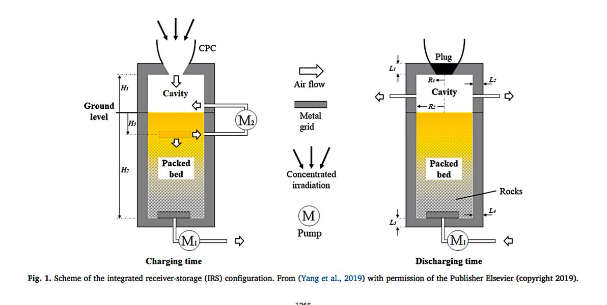
Conceptual design of an integrated solar receiver and thermal energy storage system, relevant if "GHS" implies Gas Heat Storage.
Modeling the Heat Transfer Fluid (Gas)
Thermophysical Properties
The properties of the gas (density \(\rho\), specific heat capacity \(c_p\), thermal conductivity \(k_{gas}\), viscosity \(\mu\)) are crucial. For gases, these properties are strongly dependent on temperature and, to a lesser extent, pressure. Accurate correlations or databases for these properties as functions of temperature are essential, especially given the wide temperature ranges experienced in GHS-CSP systems.
For example, the specific heat capacity \(c_p(T)\) might be represented by a polynomial function of temperature.
Fluid Dynamics
The flow of the gas through the receiver passages (e.g., tubes, channels in porous media) must be modeled. This involves solving equations for mass and momentum conservation (Navier-Stokes equations for viscous flow). Key aspects include:
- Pressure Drop: Calculating the pressure drop across the receiver is vital for determining pumping power requirements. This often involves friction factor correlations (e.g., Darcy-Weisbach equation).
- Flow Distribution: Ensuring uniform flow distribution is important for avoiding hot spots and achieving efficient heat transfer. Non-uniformities can significantly impact performance.
- Turbulence: At high flow rates, the gas flow is often turbulent. Turbulence models (e.g., k-epsilon, k-omega) may be needed to accurately predict heat transfer coefficients and flow behavior.
The energy equation for the fluid flow, coupling heat transfer with fluid motion, often takes the form (for incompressible flow, neglecting viscous dissipation):
\[ \rho c_p \left( \frac{\partial T}{\partial t} + \mathbf{u} \cdot \nabla T \right) = \nabla \cdot (k_{gas} \nabla T) + S_{heat} \]Where \( \mathbf{u} \) is the velocity vector of the gas and \( S_{heat} \) represents heat sources (e.g., from the receiver walls).
Receiver Geometry and Material Properties
The specific geometry of the receiver (e.g., tube diameter and length, porosity and pore size for volumetric receivers, cavity shape) heavily influences heat transfer and fluid flow. Material properties of the receiver structure (thermal conductivity, emissivity, absorptivity, mechanical strength at high temperatures, resistance to thermal shock and creep) are critical inputs. These properties can also be temperature-dependent.
Optical Modeling of Concentrated Solar Flux
Accurately determining the distribution and intensity of concentrated solar radiation on (or within) the receiver surfaces is a prerequisite for thermal modeling. This is often done using:
- Ray-tracing methods: Software like SolTrace or Tonatiuh simulates the path of individual sun rays from the concentrator field to the receiver, providing detailed flux maps.
- Analytical or semi-analytical methods: For simpler geometries, these can provide approximations of flux distribution.
The output of the optical model (i.e., the incident heat flux distribution \(q''_{solar}(x,y,z)\)) serves as a boundary condition or source term for the thermal model of the receiver.
Summary of Key Equations and Parameters
The table below summarizes some of the fundamental equations and associated parameters commonly encountered in the mathematical modeling of GHS-CSP receiver systems. This is not exhaustive but provides a quick reference to the core physics involved.
| Phenomenon | Key Equation (Simplified Form) | Parameters & Variables | Description |
|---|---|---|---|
| Energy Balance (Overall) | \( \frac{dE_{stored}}{dt} = Q_{in} - Q_{out} - Q_{loss} \) | \(E_{stored}\) (Stored Energy), \(Q\) (Heat Rates), \(t\) (Time) | Conservation of energy for a control volume. |
| Solar Radiation Absorption | \( Q_{solar\_abs} = G_{conc} \cdot A_{rec,ap} \cdot \alpha_{eff} \) | \(G_{conc}\) (Concentrated Flux), \(A_{rec,ap}\) (Aperture Area), \(\alpha_{eff}\) (Effective Absorptance) | Rate of solar energy absorbed by the receiver. |
| Convective Heat Transfer (Internal HTF) | \( Q_{conv,int} = h_{int} \cdot A_s \cdot (T_s - T_{gas}) \) | \(h_{int}\) (Internal HTC), \(A_s\) (Surface Area), \(T_s\) (Surface Temp), \(T_{gas}\) (Gas Temp) | Heat transfer from receiver surface to the gas. |
| Convective Heat Loss (External) | \( Q_{conv,loss} = h_{ext} \cdot A_s \cdot (T_s - T_{amb}) \) | \(h_{ext}\) (External HTC), \(A_s\) (Surface Area), \(T_s\) (Surface Temp), \(T_{amb}\) (Ambient Temp) | Heat loss from receiver exterior to surroundings. |
| Radiative Heat Loss | \( Q_{rad\_loss} = \epsilon \cdot \sigma \cdot A_s \cdot (T_s^4 - T_{amb}^4) \) | \(\epsilon\) (Emissivity), \(\sigma\) (Stefan-Boltzmann Const.), \(A_s\) (Surface Area), \(T_s\), \(T_{amb}\) | Heat loss by radiation from receiver surface. |
| Conduction (1D, Steady) | \( Q_{cond} = -k \cdot A_c \cdot \frac{dT}{dx} \) | \(k\) (Thermal Conductivity), \(A_c\) (Cross-section Area), \(dT/dx\) (Temp. Gradient) | Heat transfer through solid receiver materials. |
| Gas Energy Gain | \( Q_{HTF} = \dot{m}_{gas} \cdot c_{p,gas} \cdot (T_{out,gas} - T_{in,gas}) \) | \(\dot{m}_{gas}\) (Mass Flow Rate), \(c_{p,gas}\) (Specific Heat), \(T_{out,gas}, T_{in,gas}\) (Outlet/Inlet Gas Temps) | Net heat absorbed by the flowing gas. |
| Radiative Transfer Eq. (Simplified) | \( \frac{dI}{ds} = -\kappa I + \sigma_s I + \kappa I_b \) | \(I\) (Radiation Intensity), \(\kappa\) (Absorption Coeff.), \(\sigma_s\) (Scattering Coeff.), \(I_b\) (Blackbody Intensity) | Governs radiation transport within participating media (e.g., volumetric receivers, some gases). |
| Fluid Energy Equation (Simplified) | \( \rho c_p (\frac{\partial T}{\partial t} + \mathbf{u} \cdot \nabla T) = \nabla \cdot (k \nabla T) + S \) | \(\rho, c_p, k, \mathbf{u}, T, S\) (Density, Specific Heat, Conductivity, Velocity, Temperature, Source Term) | Describes temperature distribution in the flowing gas considering convection and conduction. |
Note: HTC stands for Heat Transfer Coefficient. Many parameters like \(h, k, c_p, \rho, \epsilon, \alpha\) can be temperature-dependent, adding complexity to the model.
Advanced Modeling Techniques
While the fundamental equations provide a basis, advanced computational techniques are often necessary for accurate and detailed modeling of GHS-CSP receivers, especially given their complex geometries, high operating temperatures, and coupled physical phenomena.
Computational Fluid Dynamics (CFD)
CFD has become an indispensable tool for analyzing CSP receivers. It involves numerically solving the governing equations of fluid flow (Navier-Stokes equations), heat transfer (energy equation), and sometimes radiation transport (Radiative Transfer Equation - RTE) over a discretized domain representing the receiver.
Solving Transport Equations
CFD codes (like Ansys Fluent, OpenFOAM) use methods like the Finite Volume Method (FVM) to solve these coupled, non-linear partial differential equations. For gas-phase receivers, key capabilities include:
- Modeling turbulent flow of the gas.
- Simulating conjugate heat transfer (CHT), which couples heat transfer in the fluid with conduction in the solid receiver materials.
- Incorporating models for radiative heat transfer, including surface-to-surface radiation and, for volumetric receivers or participating gases, solving the RTE using methods like the Discrete Ordinates (DO) model or P1 approximation.
- Handling complex geometries accurately.
Advantages and Applications
CFD allows for:
- Detailed prediction of temperature distributions in both the gas and solid structures, helping to identify potential hot spots or areas of poor heat transfer.
- Calculation of velocity profiles and pressure drops.
- Optimization of receiver design parameters (e.g., absorber tube arrangement, porous structure morphology, flow channel dimensions).
- Assessment of thermal performance under various operating conditions.
- Evaluation of non-uniform solar flux distributions.
Finite Element Method (FEM) for Structural Analysis
The high temperatures and significant thermal gradients experienced by CSP receivers can lead to substantial thermal stresses and strains in the materials. FEM is widely used to perform structural analysis. Temperature distributions obtained from thermal models (often CFD) can be used as input for FEM simulations to:
- Calculate thermal stresses and deformations.
- Assess the risk of mechanical failure due to yielding, fatigue (from thermal cycling), or creep (at sustained high temperatures).
- Inform material selection and structural design to ensure durability and longevity.
System-Level and Transient Simulations
For predicting the overall performance of the CSP plant over longer periods (e.g., daily or annual energy yield) and under varying solar conditions, system-level simulation tools (e.g., TRNSYS, SAM, Modelica-based environments) are used. These models typically use simplified representations (e.g., performance maps or reduced-order models derived from detailed CFD/FEM analyses) of components like the receiver. Transient simulations are crucial for:
- Analyzing start-up, shutdown, and cloud passage behavior.
- Evaluating the performance of integrated thermal energy storage systems.
- Optimizing control strategies.
Visualizing CSP Technology
To better understand the broader context in which GHS-CSP receiver models are applied, it's helpful to visualize how Concentrated Solar Power systems operate. The following video provides a general overview of CSP technology, illustrating how sunlight is concentrated and converted into usable energy. This foundational knowledge helps appreciate the role and complexity of the receiver component.
This video explains the basic principles of CSP, showcasing how mirrors focus sunlight onto a receiver. While it may not specifically detail gas-phase receivers, it lays the groundwork for understanding why efficient and robust receiver design, guided by mathematical modeling, is so critical to the success of CSP technology.
Frequently Asked Questions (FAQ)
What does "GHS" likely stand for in the context of CSP receivers?
While "GHS" is not a universally standard acronym in CSP, in the context of "GHS on a CSP receiver," it most plausibly refers to systems involving gas. This primarily points towards:
- Gas-Phase Solar Receivers: These receivers use a gas (like air, helium, or CO₂) as the heat transfer fluid. They are designed to achieve very high temperatures.
- Gas Heat Storage: This could refer to thermal energy storage systems that use gas as the medium to transport heat to and from a solid storage material (e.g., packed beds of rocks or ceramics).
The common thread is the use of gas in high-temperature applications within the CSP system, either for direct heat transfer in the receiver or for thermal storage.
Why are gases used as heat transfer fluids in some CSP systems?
Gases offer several potential advantages as heat transfer fluids in CSP systems, especially for achieving high temperatures:
- High-Temperature Stability: Gases like air, helium, or CO₂ can operate at much higher temperatures (e.g., >700°C, even >1000°C) than traditional HTFs like molten salts (typically limited to around 550-600°C) without decomposing.
- Power Cycle Integration: Hot gas can directly drive high-efficiency gas turbines (Brayton cycle), potentially leading to higher overall plant efficiencies.
- Availability and Cost: Air, for example, is readily available and free, though its heat transfer properties are not as good as other gases or liquids.
- Reduced Corrosion Issues: Some gases can be less corrosive to piping and receiver materials compared to molten salts at high temperatures.
- Applications Beyond Electricity: High-temperature gas can be used for industrial process heat or to drive thermochemical reactions for solar fuel production.
However, gases also have challenges, such as lower volumetric heat capacity and lower heat transfer coefficients compared to liquids, often requiring larger heat exchangers or specialized receiver designs (like volumetric receivers) and higher pumping power.
What are the main challenges in modeling GHS-CSP systems?
Modeling GHS-CSP systems presents several significant challenges:
- Extreme Temperatures: Accurately modeling material properties (thermal, optical, mechanical) and heat transfer phenomena at very high temperatures (often >700°C) is complex, as properties can change significantly.
- Coupled Physics: The models must often handle tightly coupled phenomena, including fluid dynamics, multi-mode heat transfer (conduction, convection, radiation), and structural mechanics (thermal stresses). Radiation, in particular, becomes dominant at high temperatures and can be computationally intensive to model accurately.
- Complex Geometries: Modern receiver designs, especially volumetric receivers or those with intricate flow paths, require detailed geometric representation and meshing for numerical simulations.
- Transient Behavior: Solar input is inherently variable. Modeling the transient response of the receiver and any integrated storage to changes in solar radiation, ambient conditions, or load demands is crucial for performance prediction and control system design.
- Material Degradation: High temperatures, thermal cycling, and potentially harsh chemical environments (if gases are not inert) can lead to material degradation (e.g., oxidation, creep). Predicting these effects and their impact on performance and lifetime is a significant modeling challenge.
- Validation: Obtaining high-quality experimental data from high-temperature gas-phase CSP systems for model validation can be difficult and expensive.
How does CFD help in designing CSP receivers?
Computational Fluid Dynamics (CFD) is a powerful tool in the design and optimization of CSP receivers, including gas-phase systems, by enabling detailed simulations of thermo-fluid phenomena. Its contributions include:
- Flow Visualization and Analysis: CFD provides detailed insights into the gas flow patterns, velocity distributions, and pressure drops within the receiver. This helps identify areas of stagnation, recirculation, or non-uniform flow that could impair performance.
- Temperature Distribution Mapping: It can predict precise temperature distributions in both the gas and the solid receiver materials. This is critical for identifying potential hot spots that could lead to material failure or cold spots that reduce efficiency.
- Heat Transfer Optimization: CFD allows designers to evaluate the effectiveness of different heat transfer enhancement techniques and optimize geometric parameters (e.g., tube spacing, porous media structure) to maximize heat absorption by the gas and minimize losses.
- Flux Distribution Impact: It can simulate the effect of non-uniform incident solar flux on the receiver's thermal performance and temperature uniformity.
- Parametric Studies & Design Iteration: Designers can use CFD to conduct virtual experiments, rapidly testing different design variations and operating conditions to arrive at an optimized design before building expensive prototypes.
- Conjugate Heat Transfer (CHT): CFD can simultaneously model heat transfer in the fluid and conduction in the solid parts of the receiver, providing a comprehensive thermal analysis.
- Radiative Heat Transfer Modeling: Advanced CFD models include solvers for the Radiative Transfer Equation (RTE), crucial for accurately predicting radiative exchange within cavities or participating media at high temperatures.
By providing such detailed information, CFD helps to improve receiver efficiency, enhance durability, reduce development costs, and mitigate risks associated with high-temperature operation.
Can these models predict the lifespan of a CSP receiver?
While the primary focus of the thermo-fluid models discussed is on performance (temperature, efficiency, heat loss), they provide crucial inputs for lifespan prediction. Lifespan assessment itself is a complex, multi-faceted problem that typically involves additional modeling layers:
- Thermal Stress Analysis: Temperature distributions predicted by CFD or other thermal models are fed into Finite Element Method (FEM) structural models. These FEM models calculate thermal stresses and strains caused by temperature gradients and thermal cycling (daily start-up/shutdown, cloud transients).
- Material Degradation Models:
- Creep: At sustained high temperatures, materials can undergo creep deformation, which can lead to rupture. Creep models (e.g., based on Larson-Miller parameters or Norton's Law) use temperature and stress data to predict creep damage accumulation over time.
- Fatigue: Thermal cycling induces cyclic stresses, which can lead to fatigue failure. Fatigue life models (e.g., S-N curves, strain-life approaches like Coffin-Manson) use the history of stress/strain cycles to predict fatigue damage.
- Oxidation/Corrosion: High temperatures and the operating environment (e.g., air as HTF) can cause oxidation or corrosion of receiver materials, thinning components or altering their properties. Models for these chemical degradation mechanisms can predict material loss rates.
- Damage Accumulation Rules: Combined damage from creep and fatigue is often assessed using rules like linear damage summation (e.g., Miner's rule for fatigue).
So, while a single GHS thermal model doesn't directly output "lifespan," it's a critical first step. By providing accurate temperature and heat flux data, these models enable subsequent structural and material degradation analyses that are essential for estimating the operational lifetime of a CSP receiver and identifying critical components or failure modes.
Recommended Further Exploration
To delve deeper into the fascinating world of Concentrated Solar Power and high-temperature receiver modeling, consider exploring these related topics:
- How is Computational Fluid Dynamics specifically applied to model volumetric solar receivers that use porous media for heat absorption?
- What are the primary materials science challenges and solutions for developing CSP receivers capable of sustained operation above 800°C?
- What are the key aspects of dynamic modeling and control strategies for CSP plants that integrate thermal energy storage to ensure stable power output?
- How do different gas heat transfer fluids (like air, helium, CO₂) compare in terms of performance, cost, and system implications for high-temperature CSP applications?
References
The information presented is synthesized from general knowledge in the field and informed by concepts discussed in the following types of resources:
Last updated May 19, 2025