
Spatial Pythagorean Hodograph Curves: Theory and MATLAB Implementation
A comprehensive guide to spatial PH curves and example MATLAB code
Key Takeaways
- Exact Arc Length Computation: Spatial PH curves allow for precise and efficient computation of arc lengths without numerical integration.
- Quaternion-Based Formulation: Their construction in 3D often involves quaternions to ensure the Pythagorean property and satisfy boundary conditions.
- Practical MATLAB Implementation: MATLAB code frameworks exist that interpolate between given starting and ending positions and directions while ensuring the PH property.
Introduction
Spatial Pythagorean Hodograph (PH) curves represent a special category of polynomial curves in three-dimensional space that exhibit a unique mathematical structure. The distinguishing characteristic is that the square of the magnitude of the curve’s derivative vector (also known as the "hodograph") is itself the square of a polynomial. This remarkable property implies that the speed function of the curve can be expressed exactly as a polynomial, which in turn enables exact computations of arc lengths. Applications of spatial PH curves span advanced fields such as computer-aided design (CAD), computer-aided manufacturing (CAM), robotics, path planning, motion control, and computer animation.
Unlike ordinary polynomial curves, spatial PH curves offer the added advantage of producing rational offset curves and maintaining rational unit tangent vectors. These attributes are particularly important when designing curves that satisfy strict geometric constraints. The development of these curves relies on establishing a set of free parameters and algebraic constraints that guarantee both interpolation fidelity and the Pythagorean condition. Over the years, many researchers – including Farouki and his collaborators – have contributed to the theoretical underpinnings and practical implementations of these curves.
What are Spatial PH Curves?
A spatial PH curve is typically defined as a polynomial curve r(t) = (x(t), y(t), z(t)) with the property that the squared norm of its derivative r′(t) is a perfect square of another polynomial. Mathematically, if one sets
$$|r'(t)|^2 = \sigma^2(t),$$
where σ(t) is a polynomial, then the curve possesses the Pythagorean hodograph property. This Pythagorean structure not only simplifies the computation of the arc length but also means that the offset curves constructed from these PH curves remain rational. In three-dimensional space, the construction tends to be more intricate compared to its planar counterpart due to the increased degrees of freedom.
Mathematical Foundations
The mathematical formulation underlying PH curves involves choosing an appropriate representation for r′(t). One popular approach is to express the derivative using quaternion polynomials. Consider a quaternion polynomial Q(t) = u(t) + v(t)i + w(t)j + z(t)k. By setting the derivative as:
$$r'(t) = Q(t) \, i \, \overline{Q(t)},$$
one can show through the properties of quaternions that the squared speed becomes:
$$|r'(t)|^2 = \left(|Q(t)|^2\right)^2.$$
This equation highlights that if Q(t) is chosen as a polynomial, then the speed is a polynomial squared. Such a representation is crucial to maintain the PH property. Given specific boundary conditions – namely, the starting and ending positions as well as the tangent directions – the free parameters within Q(t) can be resolved either by solving a system of polynomial equations or by employing optimization techniques.
Properties and Advantages of PH Curves
Benefits and Key Attributes
Spatial PH curves are not only theoretically elegant but also practically beneficial. Below is an HTML table summarizing the significant properties, advantages, and typical applications of these curves:
| Property | Advantage | Application |
|---|---|---|
| Exact Arc Length | Enables efficient and accurate computation without numerical integration | Motion planning, CNC machining |
| Rational Offset Curves | Simplifies tool-path generation and other CAD/CAM operations | Surface modeling, path offsetting |
| Smooth Interpolation | Provides smooth transitions between points with prescribed tangents | Robotics, computer animation |
| Quaternion Representation | Facilitates handling the complex geometry in three dimensions | 3D curve design and simulation |
Advantages in Practical Applications
One of the key benefits of spatial PH curves is their ability to produce curves with exactly computable arc lengths. This characteristic is very useful in robotics and CNC applications where precision is paramount. Furthermore, the use of quaternion polynomials in their formulation allows these curves to accommodate complex spatial orientations while still adhering to the prescribed geometric constraints. As a result, spatial PH curves are widely preferred in scenarios where maintaining smoothness and continuity is critical.
Additionally, the inherent structure of PH curves guarantees that both the unit tangent and offset curves will remain rational, which simplifies many downstream geometric computations in automated design and manufacturing processes. This property reduces computational overhead and enhances the robustness of the algorithms used in these applications.
MATLAB Implementation of Spatial PH Curves
Approach Overview
Implementing spatial PH curves in MATLAB typically involves setting up a parametric representation where the curve r(t) is computed by integrating a specially structured derivative function r′(t). The key idea is to choose polynomial representations for the derivative components that naturally satisfy the Pythagorean condition. In practice, the implementation is usually split into two main tasks:
- Defining the Polynomial Structure: Choose appropriate polynomial functions (often represented using quaternions) to define the derivative r′(t) and guarantee that its squared norm is a perfect square.
- Interpolating Boundary Conditions: Solve for the free parameters so that r(t) matches the given starting and ending positions and tangent directions. These conditions are typically denoted as r(0) = P₀, r(1) = P₁, r′(0) = d₀, and r′(1) = d₁.
A common approach is to initially represent r(t) as a polynomial expression of a fixed degree (often quintic, for its balance between flexibility and computational efficiency). The coefficients of this polynomial are then determined based on the interpolation constraints. In a more advanced treatment, the quaternion formulation is introduced, and the unknown quaternion coefficients are solved such that the PH property is preserved throughout.
Boundary Conditions and Interpolation
Let us denote the starting position by P₀ and the ending position by P₁. Similarly, the starting and ending tangent vectors are denoted by d₀ and d₁, respectively. In the most straightforward implementation, the curve r(t) is expressed as:
r(t) = C₀ + C₁t + C₂t² + C₃t³ + C₄t⁴ + C₅t⁵,
where:
- C₀ = P₀
- C₁ = d₀ (matching the starting tangent)
- C₂, C₃, C₄, C₅ – are free parameters that can be determined by imposing r(1) = P₁ and r′(1) = d₁.
Given the extra degrees of freedom associated with a quintic polynomial, one can choose some parameters arbitrarily (or based on additional optimization criteria) and solve for the remaining coefficients to meet the interpolation and Pythagorean constraints.
Quaternion Representation
Another robust method to enforce the PH condition is to represent the derivative using a quaternion polynomial Q(t). In this approach, once Q(t) is defined, the derivative is computed using the formula:
r′(t) = Q(t)·i·conjugate(Q(t)),
ensuring that:
|r′(t)|² = (|Q(t)|²)².
This formulation leverages the algebraic properties of quaternions to maintain the Pythagorean structure, even in complex three-dimensional scenarios.
MATLAB Code Example
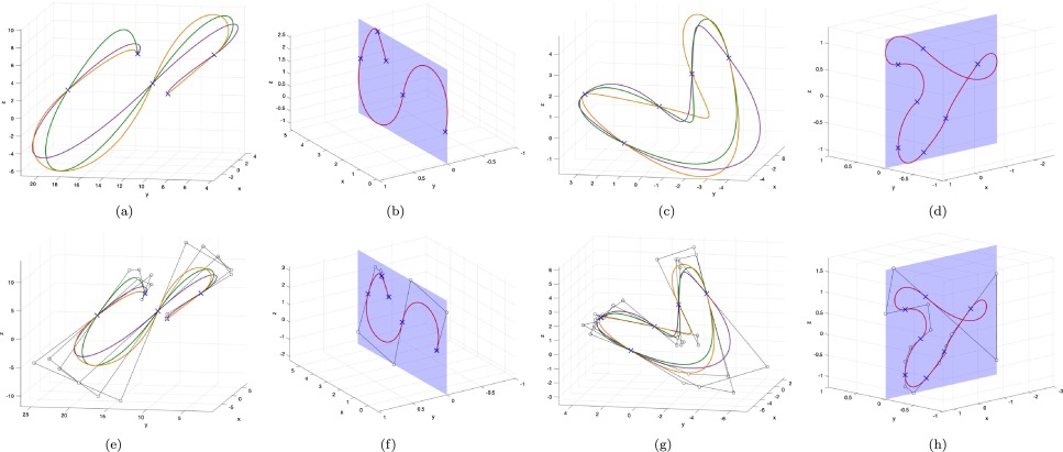
The MATLAB code below provides a basic framework for computing a spatial PH curve given the starting position, starting direction, end position, and end direction. In this example, we assume a quintic polynomial representation for the curve:
% Spatial PH Curve Computation in MATLAB
% This code computes a quintic PH curve based on given boundary conditions.
% The PH property is maintained by an appropriate choice of free parameters.

function PH_curve = computeSpatialPH(start_pos, start_dir, end_pos, end_dir)
    % Inputs:
    %   start_pos : [x0; y0; z0] -- starting position
    %   start_dir : [dx0; dy0; dz0] -- starting tangent direction (nonzero vector)
    %   end_pos   : [x1; y1; z1] -- ending position
    %   end_dir   : [dx1; dy1; dz1] -- ending tangent direction (nonzero vector)

    % We assume a quintic polynomial representation of the form:
    %   r(t) = C0 + C1*t + C2*t.^2 + C3*t.^3 + C4*t.^4 + C5*t.^5, for t in [0,1]
    % where we impose:
    %   C0 = start_pos, C1 = start_dir.
    % The coefficients C2, C3, C4, and C5 will be determined from the conditions:
    %   r(1) = end_pos, and r'(1) = end_dir.

    % Set C0 and C1
    C0 = start_pos;
    C1 = start_dir;

    % Introduce free parameters for C2 and C3 (user can choose these based on design criteria)
    A = [0.5; 0; 0.1];
    B = [0; 0.5; 0.0];
    C2 = A;
    C3 = B;

    % The remaining coefficients, C4 and C5, are determined by enforcing the endpoint conditions.
    % r(1) = C0 + C1 + C2 + C3 + C4 + C5 should equal end_pos.
    % r'(1) = C1 + 2*C2 + 3*C3 + 4*C4 + 5*C5 should equal end_dir.
    %
    % We can express C5 as:
    %   C5 = end_pos - (C0 + C1 + C2 + C3 + C4)
    % Substitute r'(1) condition and solve for C4:
    %   C1 + 2*C2 + 3*C3 + 4*C4 + 5*(end_pos - (C0 + C1 + C2 + C3 + C4)) = end_dir
    % Rearranging gives:
    %   C4 = C1 + 2*C2 + 3*C3 - 5*(C1+C2+C3) + 5*(end_pos-C0) - end_dir;

    C4 = C1 + 2*A + 3*B - 5*(C1 + A + B) + 5*(end_pos - C0) - end_dir;
    C5 = end_pos - (C0 + C1 + A + B + C4);

    % Define the time domain
    t = linspace(0,1,200);

    % Preallocate the curve array
    PH_curve = zeros(3, length(t));

    % Evaluate the polynomial curve at each parameter value
    for idx = 1:length(t)
        t_val = t(idx);
        PH_curve(:,idx) = C0 + C1*t_val + A*t_val.^2 + B*t_val.^3 + C4*t_val.^4 + C5*t_val.^5;
    end

    % Optionally, plot the PH curve
    figure;
    subplot(1,2,1);
    plot3(PH_curve(1,:), PH_curve(2,:), PH_curve(3,:), 'b', 'LineWidth', 2);
    grid on; hold on;
    plot3(C0(1), C0(2), C0(3), 'ro', 'MarkerSize', 10, 'MarkerFaceColor', 'r'); % Start point
    plot3(end_pos(1), end_pos(2), end_pos(3), 'go', 'MarkerSize', 10, 'MarkerFaceColor', 'g'); % End point
    xlabel('x'); ylabel('y'); zlabel('z');
    title('Spatial PH Curve');
    legend('Curve', 'Start', 'End'); axis equal;

    subplot(1,2,2);
    % Compute and plot the speed profile |r''(t)| for verification
    speed = zeros(size(t));
    for idx = 1:length(t)
        % Derivative of the quintic polynomial
        rprime = C1 + 2*A*t(idx) + 3*B*t(idx)^2 + 4*C4*t(idx)^3 + 5*C5*t(idx)^4;
        speed(idx) = norm(rprime);
    end
    plot(t, speed, 'k', 'LineWidth', 2);
    xlabel('t'); ylabel('Speed |r''(t)|');
    title('Speed Profile');
    grid on;
end

% Example usage:
start_pos = [0; 0; 0];
start_dir = [3; 0; 1];
end_pos   = [10; 5; 3];
end_dir   = [2; 4; 0];
PH_curve = computeSpatialPH(start_pos, start_dir, end_pos, end_dir);
This MATLAB script defines a function that interpolates between given start and end conditions using a quintic polynomial form. Notice that while the free parameters A and B are arbitrarily chosen here, a more complete implementation would involve solving a system of nonlinear equations to guarantee the PH property (i.e., ensuring the squared norm of the derivative is a perfect square) throughout the curve. Advanced techniques may involve iterative refinement or optimization routines (such as MATLAB’s fsolve) to determine these parameters more accurately.
Practical Considerations
Parameter Selection and Optimization
In practical applications, the choice of free parameters (e.g., A and B in the sample code) plays a crucial role in the overall shape and fairness of the resulting spatial PH curve. Rather than selecting these parameters arbitrarily, it is common to employ optimization techniques that minimize curvature variation or other fairness measures while still satisfying the PH property. For instance, nonlinear solvers or specialized interpolation algorithms can optimize the free parameters so that the transition between the start and end conditions is as smooth as possible.
Additionally, depending on the application—whether it is robotics, animation, or CNC programming—different weighting criteria may be applied to ensure that the computed curve adheres to the desired kinematic or geometric constraints. The flexibility provided by the extra degrees of freedom in quintic or higher-order PH curves allows for such refinements without sacrificing the core advantages of having an exact arc length function.
Applications of Spatial PH Curves
Spatial PH curves are widely used in various fields due to their favorable geometric properties:
- Computer-Aided Design (CAD) and Manufacturing (CAM): They are used to create smooth, controllable curves for designing complex surfaces and machining paths where precision is vital.
- Robotics and Motion Planning: The exact computation of arc length and smooth transitions make these curves ideal for planning paths that require precise control over speed and acceleration.
- Computer Animation and Graphics: In scenarios requiring smooth transitions and natural motion, spatial PH curves offer a robust framework for generating trajectories that are both visually appealing and mathematically tractable.
- Tool Path Generation: The rationality of the offset curves derived from PH curves simplifies the complex task of generating tool paths in CNC machining, ensuring that offsets remain precise and computationally efficient.
Conclusion
Spatial Pythagorean Hodograph curves represent a sophisticated yet practical tool in computational geometry and design. Their unique property—that the squared norm of the derivative is a perfect square—allows for closed-form computations of arc length and facilitates the construction of rational offset curves. By leveraging the quaternion-based formulation and carefully interpolating the boundary conditions (starting and ending positions and tangents), it is possible to derive a spatial PH curve that meets stringent geometrical and kinematic requirements. The MATLAB code provided offers a basic framework for such computations, though further refinements and optimizations are typically necessary for industrial applications.
Overall, spatial PH curves serve not only as an elegant theoretical construct but also as a practical solution in fine-tuning motion trajectories, enhancing manufacturing precision, and ensuring smooth transitions in various engineering applications.
References
-
Spatial PH Curve Article - ScienceDirect
- Farouki Spatial PH GitHub - GitHub
- Farouki and Sakkalis Article - Springer
-
PH Curve Interpolation - ScienceDirect
- PH Curves on arXiv - arXiv
More Topics
Last updated February 19, 2025