
Maxwell's Equations: Formulations, Python Implementations, and Comparative Analysis
Introduction
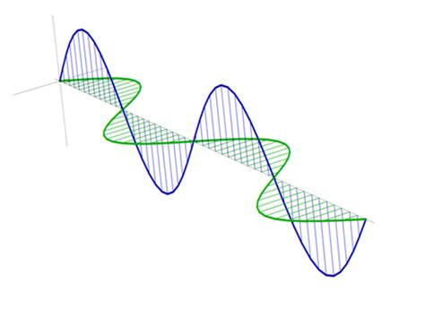
Maxwell's Equations are the cornerstone of classical electromagnetism, encapsulating how electric and magnetic fields interact and propagate. These four fundamental equations describe the behavior of electric charges, electric fields, magnetic fields, and how they influence each other. Understanding Maxwell's Equations is essential for fields ranging from electrical engineering to modern physics.
Mathematical Formulation of Maxwell's Equations
1. Gauss's Law for Electricity
Gauss's Law for Electricity relates the electric field to the distribution of electric charge. It has both differential and integral forms:
Differential Form: $$\nabla \cdot \mathbf{E} = \frac{\rho}{\varepsilon_0}$$
Integral Form: $$\oint_S \mathbf{E} \cdot d\mathbf{A} = \frac{Q_{\text{enc}}}{\varepsilon_0}$$
- Where:
- \(\nabla \cdot \mathbf{E}\): Divergence of the electric field
- \(\rho\): Charge density
- \(\varepsilon_0\): Permittivity of free space
- \(Q_{\text{enc}}\): Enclosed electric charge
- Physical Interpretation: The electric flux through a closed surface is proportional to the enclosed electric charge.
2. Gauss's Law for Magnetism
Gauss's Law for Magnetism states that there are no magnetic monopoles; magnetic field lines are continuous loops.
Differential Form: $$\nabla \cdot \mathbf{B} = 0$$
Integral Form: $$\oint_S \mathbf{B} \cdot d\mathbf{A} = 0$$
- Physical Interpretation: There are no isolated north or south magnetic poles; magnetic field lines always form closed loops.
3. Faraday's Law of Induction
Faraday's Law describes how a time-varying magnetic field induces an electric field.
Differential Form: $$\nabla \times \mathbf{E} = -\frac{\partial \mathbf{B}}{\partial t}$$
Integral Form: $$\oint_{\partial S} \mathbf{E} \cdot d\mathbf{l} = -\frac{d\Phi_B}{dt}$$
- Where:
- \(\nabla \times \mathbf{E}\): Curl of the electric field
- \(\frac{\partial \mathbf{B}}{\partial t}\): Time rate of change of the magnetic field
- \(\Phi_B\): Magnetic flux
- Physical Interpretation: A changing magnetic field induces a circulating electric field.
4. Ampère-Maxwell Law
The Ampère-Maxwell Law extends Ampère's Law by incorporating the displacement current, accounting for time-varying electric fields.
Differential Form: $$\nabla \times \mathbf{B} = \mu_0 \mathbf{J} + \mu_0 \varepsilon_0 \frac{\partial \mathbf{E}}{\partial t}$$
Integral Form: $$\oint_{\partial S} \mathbf{B} \cdot d\mathbf{l} = \mu_0 I_{\text{enc}} + \mu_0 \varepsilon_0 \frac{d\Phi_E}{dt}$$
- Where:
- \(\nabla \times \mathbf{B}\): Curl of the magnetic field
- \(\mu_0\): Permeability of free space
- \(\mathbf{J}\): Current density
- \(\frac{\partial \mathbf{E}}{\partial t}\): Time rate of change of the electric field
- \(I_{\text{enc}}\): Enclosed current
- \(\Phi_E\): Electric flux
- Physical Interpretation: Both electric currents and changing electric fields generate circulating magnetic fields.
Python Implementation: Finite-Difference Time-Domain (FDTD) Method
The Finite-Difference Time-Domain (FDTD) method is a powerful numerical technique used to solve Maxwell's Equations. Below is a comprehensive Python implementation simulating electromagnetic wave propagation in a 1D space.
Python Code Example
python import numpy as np import matplotlib.pyplot as plt # Constants epsilon_0 = 8.854e-12 # Permittivity of free space (F/m) mu_0 = 4 * np.pi * 1e-7 # Permeability of free space (H/m) c = 1 / np.sqrt(epsilon_0 * mu_0) # Speed of light (m/s) # Simulation parameters nx = 200 # Number of spatial points nt = 1000 # Number of time steps dx = 1e-3 # Spatial step size (m) dt = dx / (2 * c) # Time step size (s) - Courant condition # Field initialization Ez = np.zeros(nx) # Electric field Hy = np.zeros(nx-1) # Magnetic field # Source parameters source_position = nx // 2 source_width = 20 # Time-stepping loop for n in range(nt): # Update magnetic field for i in range(nx-1): Hy[i] += (dt / (mu_0 * dx)) * (Ez[i+1] - Ez[i]) # Update electric field for i in range(1, nx): Ez[i] += (dt / (epsilon_0 * dx)) * (Hy[i] - Hy[i-1]) # Gaussian pulse source Ez[source_position] += np.exp(-0.5 * ((n - source_width)/ (source_width / 4))**2) # Plotting at intervals if n % 100 == 0: plt.figure(figsize=(10, 4)) plt.subplot(121) plt.plot(Ez, label='Ez') plt.title('Electric Field (Ez)') plt.xlabel('Position') plt.ylabel('Ez (V/m)') plt.ylim(-1, 1) plt.legend() plt.subplot(122) plt.plot(Hy, label='Hy', color='orange') plt.title('Magnetic Field (Hy)') plt.xlabel('Position') plt.ylabel('Hy (A/m)') plt.ylim(-1, 1) plt.legend() plt.tight_layout() plt.show() ```
Explanation of the Python Code
- Constants: Defines the fundamental physical constants, including permittivity (\(\varepsilon_0\)), permeability (\(\mu_0\)), and the speed of light (\(c\)).
- Simulation Parameters: Sets the number of spatial points (\(nx\)), number of time steps (\(nt\)), spatial step size (\(dx\)), and time step size (\(dt\)), ensuring stability through the Courant condition (\(dt \leq \frac{dx}{2c}\)).
- Field Initialization: Initializes the electric field (\(E_z\)) and magnetic field (\(H_y\)) as zero arrays.
- Source Parameters: Defines the position and width of the Gaussian pulse source that injects energy into the system.
-
Time-Stepping Loop:
- Updates the magnetic field based on the spatial derivative of the electric field.
- Updates the electric field based on the spatial derivative of the magnetic field.
- Injects a Gaussian pulse at the source position to simulate an electromagnetic wave.
- Plots the fields at specified intervals to visualize the propagation.
Comparative Analysis of Maxwell's Equations
Comparison Table
| Equation | Differential Form | Integral Form | Physical Interpretation |
|---|---|---|---|
| Gauss's Law (Electric) | $$\nabla \cdot \mathbf{E} = \frac{\rho}{\varepsilon_0}$$ | $$\oint_S \mathbf{E} \cdot d\mathbf{A} = \frac{Q_{\text{enc}}}{\varepsilon_0}$$ | The electric flux through a closed surface is proportional to the enclosed electric charge. |
| Gauss's Law (Magnetic) | $$\nabla \cdot \mathbf{B} = 0$$ | $$\oint_S \mathbf{B} \cdot d\mathbf{A} = 0$$ | There are no isolated magnetic poles; magnetic field lines form closed loops. |
| Faraday's Law of Induction | $$\nabla \times \mathbf{E} = -\frac{\partial \mathbf{B}}{\partial t}$$ | $$\oint_{\partial S} \mathbf{E} \cdot d\mathbf{l} = -\frac{d\Phi_B}{dt}$$ | A changing magnetic field induces a circulating electric field. |
| Ampère-Maxwell Law | $$\nabla \times \mathbf{B} = \mu_0 \mathbf{J} + \mu_0 \varepsilon_0 \frac{\partial \mathbf{E}}{\partial t}$$ | $$\oint_{\partial S} \mathbf{B} \cdot d\mathbf{l} = \mu_0 I_{\text{enc}} + \mu_0 \varepsilon_0 \frac{d\Phi_E}{dt}$$ | Both electric currents and changing electric fields generate magnetic fields. |
Advanced Python Implementations and Libraries
Beyond the basic FDTD implementation, several Python packages and resources facilitate more sophisticated simulations of Maxwell's Equations:
-
GMES: GIST Maxwell's Equations Solver
- A Python package designed for solving Maxwell's Equations using the FDTD method.
- Features object-oriented design and supports various electromagnetic simulations.
- Available on GitHub.
-
Meep
- An open-source finite-difference time-domain (FDTD) simulation software package developed for three-dimensional simulations of electromagnetic systems.
- Comprehensive documentation and community support.
- Accessible at Meep Documentation.
-
Example Python Notebook for 2D Maxwell Solver
-
An illustrative implementation of a two-dimensional Maxwell Solver using FDTD.
- 2D Maxwell Solver Notebook
-
-
Research Articles and Resources
GMES Research Paper
semanticscholar.org
GeeksforGeeksgeeksforgeeks.org
Conclusion
Maxwell's Equations provide a comprehensive framework for understanding electromagnetic phenomena. Through both their mathematical formulations and computational implementations using Python, they offer deep insights into the behavior of electric and magnetic fields. The FDTD method, as demonstrated, is a versatile tool for simulating these equations, enabling practical applications in engineering and physics. Leveraging advanced libraries and resources can further enhance the simulation capabilities and facilitate more complex electromagnetic analyses.
Last updated January 7, 2025